📖 Fundamentals of optimization#
⏱ | words
Screencast of the end of the Monday lecture that I didn’t cover

References and additional materials
Chapters 12.2, 12.3, 12.4, 12.5, 13.4, 29.2, 30.1
Chapters 1.2.6, 1.2.7, 1.2.8, 1.2.9, 1.2.10, 1.4.1, Section 3
Basic concepts#
Definition
Consider a function \(f: A \to \mathbb{R}\) where \(A \subset \mathbb{R}^n\). A point \(x^* \in A\) is called a
maximizer of \(f\) on \(A\) if \(f(x^*) \geq f(x)\) for all \(x \in A\)
minimizer of \(f\) on \(A\) if \(f(x^*) \leq f(x)\) for all \(x \in A\)
Function \(f\) achieves its maximum value (maximum) at maximizers
Function \(f\) achieves its minimal value (minimum) at minimizers
We’ll define these concepts more formally later. For now, note the complexity of the simple idea of finding the maximum or minimum of a function and where it is achieved. The issues include:
existence of maximizers/minimizers
uniqueness of maximizers/minimizers
characterization of maximizers/minimizers (how to find, how to check if a real one is found)
Show code cell content
from myst_nb import glue
import matplotlib.pyplot as plt
import numpy as np

def subplots():
    "Custom subplots with axes through the origin"
    fig, ax = plt.subplots()
    # Set the axes through the origin
    for spine in ['left', 'bottom']:
        ax.spines[spine].set_position('zero')
    for spine in ['right', 'top']:
        ax.spines[spine].set_color('none')
    return fig, ax

xmin, xmax = 2, 8
xgrid = np.linspace(xmin, xmax, 200)
f = lambda x: -(x - 4)**2 + 10

xstar = 4.0
fig, ax = subplots()
ax.plot([xstar], [0],  'ro', alpha=0.6)
ax.set_ylim(-12, 15)
ax.set_xlim(-1, 10)
ax.set_xticks([2, xstar, 6, 8, 10])
ax.set_xticklabels([2, r'$x^*=4$', 6, 8, 10], fontsize=14)
ax.plot(xgrid, f(xgrid), 'b-', lw=2, alpha=0.8, label=r'$f(x) = -(x-4)^2+10$')
ax.plot((xstar, xstar), (0, f(xstar)), 'k--', lw=1, alpha=0.8)
#ax.legend(frameon=False, loc='upper right', fontsize=16)
glue("fig_maximizer", fig, display=False)

xstar = xmax
fig, ax = subplots()
ax.plot([xstar], [0],  'ro', alpha=0.6)
ax.text(xstar, 1, r'$x^{**}=8$', fontsize=16)
ax.set_ylim(-12, 15)
ax.set_xlim(-1, 10)
ax.set_xticks([2, 4, 6, 10])
ax.set_xticklabels([2, 4, 6, 10], fontsize=14)
ax.plot(xgrid, f(xgrid), 'b-', lw=2, alpha=0.8, label=r'$f(x) = -(x-4)^2+10$')
ax.plot((xstar, xstar), (0, f(xstar)), 'k--', lw=1, alpha=0.8)
#ax.legend(frameon=False, loc='upper right', fontsize=16)
glue("fig_minimizer", fig, display=False)

xmin, xmax = 0, 1
xgrid1 = np.linspace(xmin, xmax, 100)
xgrid2 = np.linspace(xmax, 2, 10)

fig, ax = subplots()
ax.set_ylim(0, 1.1)
ax.set_xlim(-0.0, 2)
func_string = r'$f(x) = x^2$ if $x < 1$ else $f(x) = 0.5$'
ax.plot(xgrid1, xgrid1**2, 'b-', lw=3, label=func_string)
ax.plot(xgrid2, -0.25 * xgrid2 + 0.5, 'b-', lw=3)
ax.plot(xgrid1[-1], xgrid1[-1]**2, marker='o', markerfacecolor='white', markeredgewidth=2, markersize=6, color='b')
ax.plot(xgrid2[0], -0.25 * xgrid2[0] + 0.5, marker='.', markerfacecolor='b', markeredgewidth=2, markersize=10, color='b')
glue("fig_none", fig, display=False)

fig, ax = subplots()
ax.set_ylim(-2.1, 20.1)
ax.set_xlim(-0.0, 2)
func_string = r'$f(x) = 1/1-x$ if $x < 1$ else $f(x) = -3x$'
ax.plot(xgrid1, 1/(1-xgrid1), 'b-', lw=3, label=func_string)
ax.plot(xgrid2, -3 * xgrid2 + 6, 'b-', lw=3)
ax.plot(xgrid2[0], -3 * xgrid2[0] + 6, marker='.', markerfacecolor='b', markeredgewidth=2, markersize=10, color='b')
glue("fig_none2", fig, display=False)
/tmp/ipykernel_2162/4109180995.py:62: RuntimeWarning: divide by zero encountered in divide
  ax.plot(xgrid1, 1/(1-xgrid1), 'b-', lw=3, label=func_string)
Example
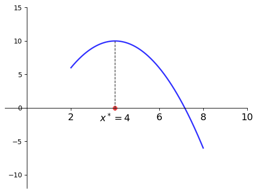
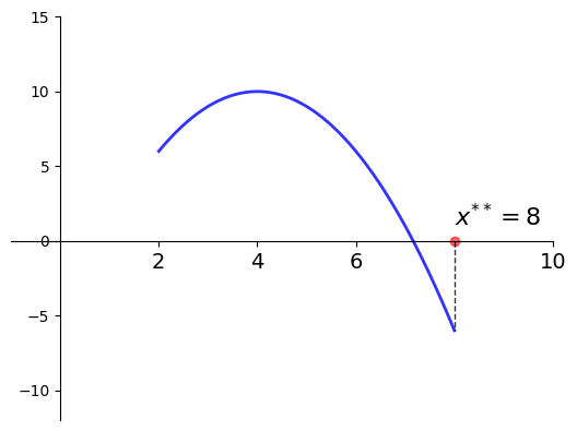
Let
\(f(x) = -(x-4)^2 + 10\)
\(a = 2\) and \(b=8\)
Then
\(x^* = 4\) is a maximizer of \(f\) on \([2, 8]\)
\(x^{**} = 8\) is a minimizer of \(f\) on \([2, 8]\)
Fig. 19 Maximizer on \([a, b] = [2, 8]\) is \(x^* = 4\)#
Fig. 20 Minimizer on \([a, b] = [2, 8]\) is \(x^{**} = 8\)#
The set of maximizers/minimizers can be
empty
a singleton (contains one element)
finite (contains a number of elements)
infinite (contains infinitely many elements)
Example: infinite maximizers
\(f \colon [0, 1] \to \mathbb{R}\) defined by \(f(x) =1\)
has infinitely many maximizers and minimizers on \([0, 1]\)
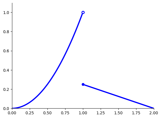
Example: no maximizers
The following function has no maximizers on \([0, 2]\)
Fig. 21 No maximizer on \([0, 2]\)#
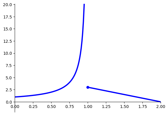
Example: no maximizers
The following function has no maximizers on \([0, 2]\)
Fig. 22 No maximizer on \([0, 2]\)#
\(\mathbb{R}^1\) univariate case#
Let \(f \colon [a, b] \to \mathbb{R}\) be a differentiable (smooth) function
Domain now is \([a, b]\) is all \(x\) with \(a \leq x \leq b\) in \(\mathbb{R}\)
\(f\) takes \(x \in [a, b]\) and returns number \(f(x)\)
derivative \(f'(x)\) exists for all \(x\) with \(a < x < b\)
Definition
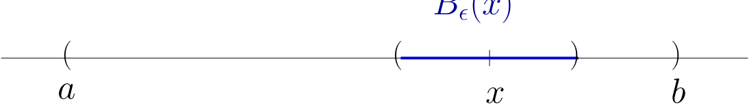
Point \(x \in \mathbb{R}\) is called interior to \([a, b]\) if \(a < x < b\)
The set of all interior points is written \((a, b)\)
We refer to \(x^* \in [a, b]\) as
interior maximizer if both a maximizer and interior
interior minimizer if both a minimizer and interior
Definition
A stationary point of \(f\) on \([a, b]\) is an interior point \(x\) with \(f'(x) = 0\)
Fact
If \(f\) is differentiable and \(x^*\) is either an interior minimizer or an interior maximizer of \(f\) on \([a, b]\), then \(x^*\) is stationary
Proof
Intuition for the proof:
Taking the linear approximation of the function \(f\) around \(x^*\) (first terms of the Taylor series)
If \(f'(x^*) \ne 0\) then exists small \(h\) such that \(f(x^* + h) > f(x^*)\) provided \(h>0\) and \(f'(x^*)>0\). \(\blacksquare\)
Converse is not true: not all stationary points are maximizers/minimizers!
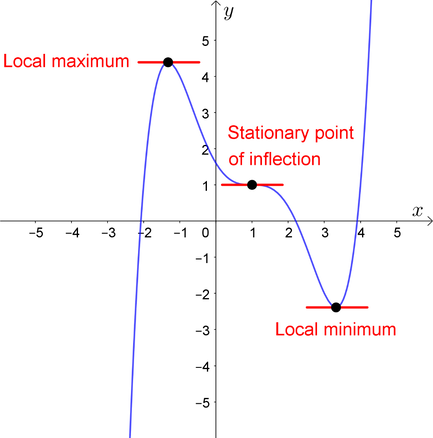
Fig. 23 Interior maximizers/minimizers are stationary points, but not all stationary points are maximizers!#
Fact
Previous fact \(\implies\)
\(\implies\) any interior maximizer is stationary
\(\implies\) set of interior maximizers \(\subset\) set of stationary points
\(\implies\) maximizers \(\subset\) stationary points \(\cup \{a,b\}\)
Algorithm for univariate problems
Locate stationary points
Evaluate \(y = f(x)\) for each stationary \(x\) and for \(a\), \(b\)
Pick the point giving largest \(y\) value
Minimization: same idea
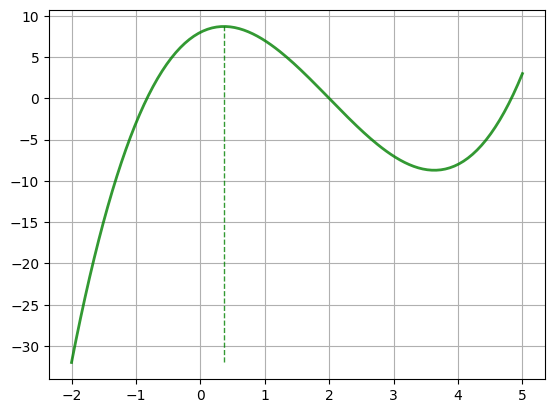
Example
Let’s solve
Steps
Differentiate to get \(f'(x) = 3x^2 - 12x + 4\)
Solve \(3x^2 - 12x + 4 = 0\) to get stationary \(x\)
Discard any stationary points outside \([-2, 5]\)
Eval \(f\) at remaining points plus end points \(-2\) and \(5\)
Pick point giving largest value
from sympy import *
x = Symbol('x')
points = [-2, 5]
f = x**3 - 6*x**2 + 4*x + 8
fp = diff(f, x)
spoints = solve(fp, x)
points.extend(spoints)
v = [f.subs(x, c).evalf() for c in points]
maximizer = points[v.index(max(v))]
print("Maximizer =", str(maximizer),'=',maximizer.evalf())
Maximizer = 2 - 2*sqrt(6)/3 = 0.367006838144548
Show code cell source
import matplotlib.pyplot as plt
import numpy as np
xgrid = np.linspace(-2, 5, 200)
f = lambda x: x**3 - 6*x**2 + 4*x + 8
fig, ax = plt.subplots()
ax.plot(xgrid, f(xgrid), 'g-', lw=2, alpha=0.8)
ax.plot((maximizer, maximizer), (f(xgrid[0]), f(maximizer)), 'g--', lw=1, alpha=0.8)
ax.grid()
Function shape and sufficiency of stationary point condition#
Preview into what we will study in detail for multivariate functions
Q: When is condition \(f'(x^*) = 0\) sufficient for \(x^*\) to be a maximizer?
A: When \(f\) is concave!
Show code cell source
xgrid = np.linspace(-2, 2, 200)
f = lambda x: - 8*x**2 + 8
fig, ax = subplots()
ax.set_ylim(-15, 10)
ax.set_yticks([-15, -10, -5, 5, 10])
ax.set_xticks([-1, 0, 1])
ax.plot(xgrid, f(xgrid), 'b-', lw=2, alpha=0.8, label='concave $f$')
ax.legend(frameon=False, loc='lower right')
plt.show()
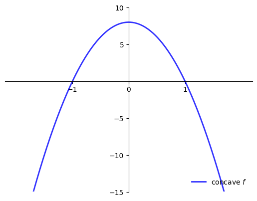
We will come back to shape conditions and full definitions of concavity/convexity later in the course.
Sufficient conditions for concavity in one dimension
Let \(f \colon [a, b] \to \mathbb{R}\)
If \(f''(x) \leq 0\) for all \(x \in (a, b)\) then \(f\) is concave on \((a, b)\)
If \(f''(x) < 0\) for all \(x \in (a, b)\) then \(f\) is strictly concave on \((a, b)\)
Example
\(f(x) = a x + b\) is concave on \(\mathbb{R}\) but not strictly
\(f(x) = \log(x)\) is strictly concave on \((0, \infty)\)
Fact
For maximizers:
If \(f \colon [a,b] \to \mathbb{R}\) is concave and \(x^* \in (a, b)\) is stationary then \(x^*\) is a maximizer
If, in addition, \(f\) is strictly concave, then \(x^*\) is the unique maximizer
Show code cell content
p = 2.0
w = 1.0
alpha = 0.6
xstar = (alpha * p / w)**(1/(1 - alpha))
xgrid = np.linspace(0, 4, 200)
f = lambda x: x**alpha
pi = lambda x: p * f(x) - w * x
fig, ax = subplots()
ax.set_xticks([1,xstar,2,3])
ax.set_xticklabels(['1',r'$\ell^*$','2','3'], fontsize=14)
ax.plot(xgrid, pi(xgrid), 'b-', lw=2, alpha=0.8, label=r'$\pi(\ell) = p\ell^{\alpha} - w\ell$')
ax.plot((xstar, xstar), (0, pi(xstar)), 'g--', lw=1, alpha=0.8)
#ax.legend(frameon=False, loc='upper right', fontsize=16)
glue("fig_price_taker", fig, display=False)
glue("ellstar", round(xstar,4))
Example
A price taking firm faces output price \(p > 0\), input price \(w >0\)
Maximize profits with respect to input \(\ell\)
where the production technology is given by
Evidently
so unique stationary point is
Moreover,
for all \(\ell \ge 0\) so \(\ell^*\) is unique maximizer.
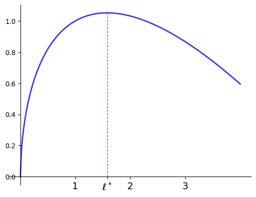
Fig. 24 Profit maximization with \(p=2\), \(w=1\), \(\alpha=0.6\), \(\ell^*=\)1.5774#
Local vs global minimizers and maximizers#
So far we have been talking about global maximizers and minimizers:
definition in the very beginning
algorithm above for univariate function on closed interval
It is important to keep in mind the desctinction between the global and local optima.
Definition
Consider a function \(f: A \to \mathbb{R}\) where \(A \subset \mathbb{R}^n\). A point \(x^* \in A\) is called a
local maximizer of \(f\) if \(\exists \delta>0\) such that \(f(x^*) \geq f(x)\) for all \(x \in B_\delta(x^*) \cap A\)
local minimizer of \(f\) if \(\exists \delta>0\) such taht \(f(x^*) \leq f(x)\) for all \(x \in B_\delta(x^*) \cap A\)
In other words, a local optimizer is a point that is a maximizer/minimizer in some neighborhood of it and not necesserily in the whole function domain.
Example
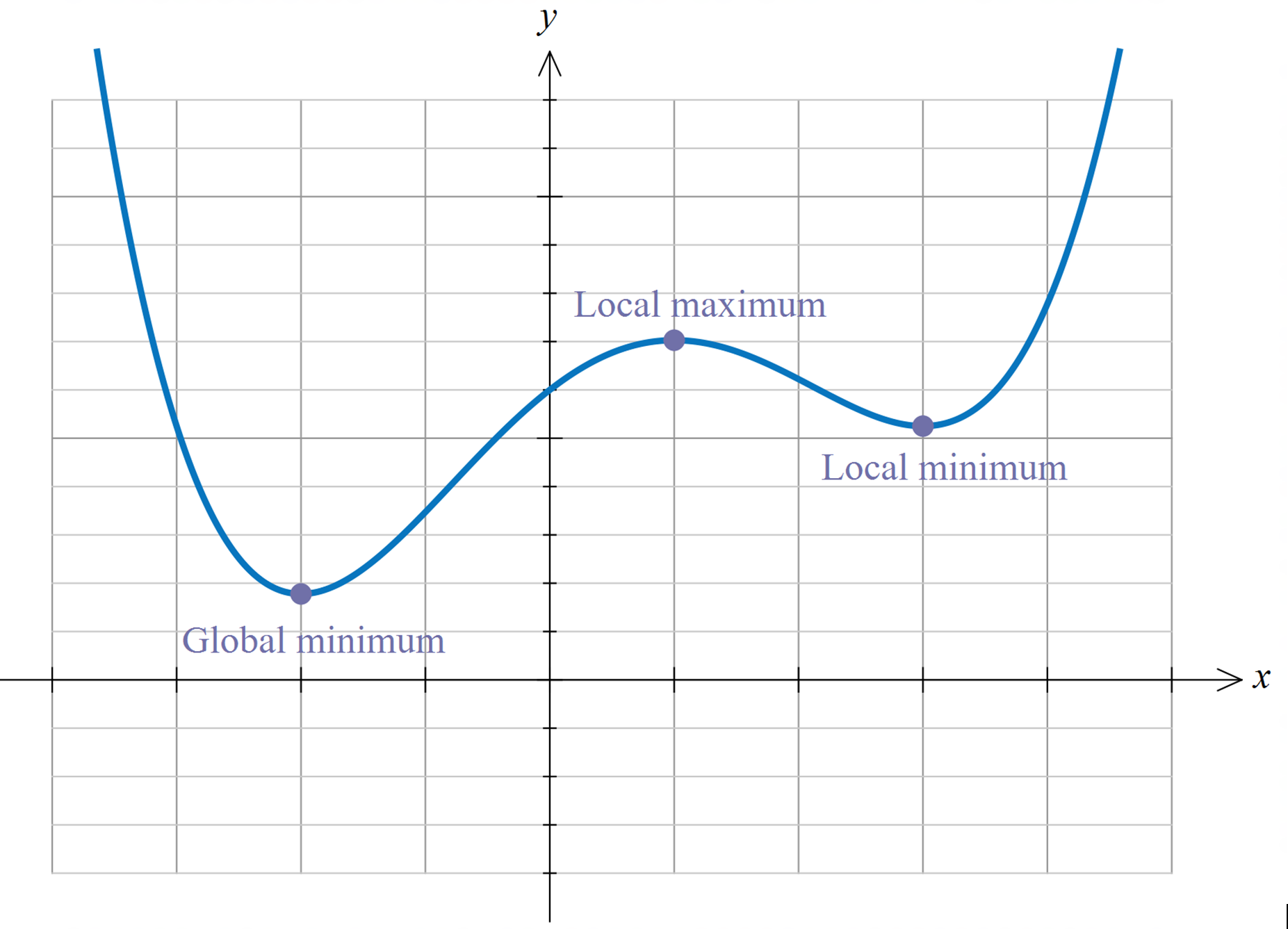
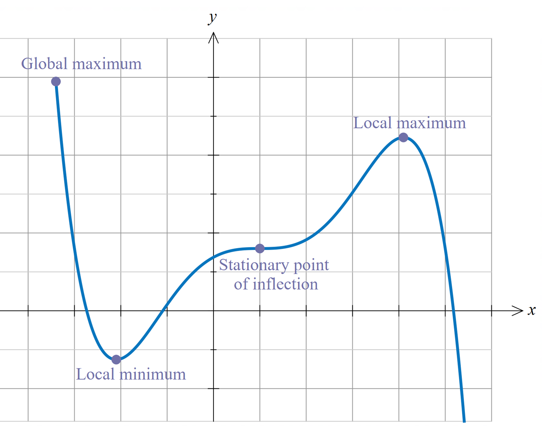
So far we have seen:
(global) maximizers and minimizers may or may not exist
stationary points are important but are neither necessary nor sufficient for finding (global) maximizers/minimizers
convexity and concavity makes stationary points sufficient for maximizers/minimizers
we have conditions for local maximizers/minimizers only, but in the univariate case can check the end points of th interval explicitly
Need rigorous theory of existance of optima!
Bounded sets#
Note
From here on transition to the multidimensional case, everything is on \(\mathbb{R}^n\) (Cartesian product of real lines \(\mathbb{R}\))
Definition
A set \(A \subset \mathbb{R}^N\) called bounded if
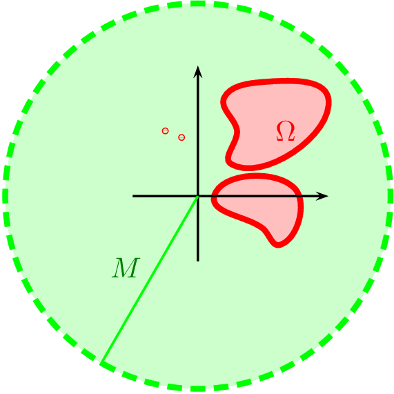
Fig. 25 Bounded set in \(\mathbb{R}^2\)#
Example
Every finite subset \(A\) of \(\mathbb{R}\) is bounded
Indeed, set \(M := \max \{ |a| : a \in A \}\). Then \(A\) is bounded by definition
Example
The set \(\{(x,y)\in\mathbb{R}^2\colon xy \leqslant 1 \}\) is unbounded
Proof:
For any \(M \in \mathbb{R}\) consider the point with coordinates \(x=1/M\) and \(y=M\). This point belongs to the set because it satisfies \(xy=1\), yet
Therefore, for any candidate bound \(M\) we can find points in the set that are further away from the origin than \(M\).
Example
Interval \((a, b)\) is bounded for any \(a, b \in \mathbb{R}\)
Proof:
Let \(M := \max\{ |a|, |b| \}\). We have to show that each \(x \in (a, b)\) satisfies \(|x| \leq M\)
Cases:
\(0 \le a \le b \implies x > 0, x = |x| < |b| = b = \max\{|a|,|b|\}\)
\(a \le b \le 0 \implies a < x < 0, |x|= -x < -a = |a| = \max\{|a|,|b|\}\)
\(a \le 0 \le b \implies\)
Fact
If \(A\) and \(B\) are bounded sets then so is \(A \cup B\)
Proof
Let \(A\) and \(B\) be bounded sets and let \(C := A \cup B\)
By definition, \(\exists \, M_A\) and \(M_B\) with
Let \(M_C := \max\{M_A , M_B\}\) and fix any \(x \in C\)
Open and closed sets#
Definition
Let \(G \subset \mathbb{R}^N\). We call \(x \in G\) interior to \(G\) if \(\exists \; \epsilon > 0\) with \(B_\epsilon(x) \subset G\)
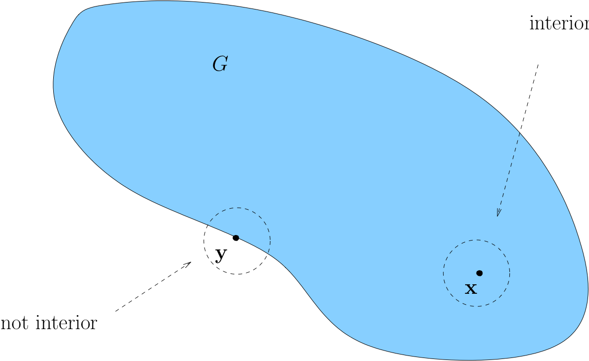
Fig. 26 Loosely speaking, interior means “not on the boundary”#
Example
Set of real numbers \(\mathbb{R}\) is open because every point is obviously interior.
Example

Example
If \(G = (a, b)\) for some \(a < b\), then any \(x \in (a, b)\) is interior
Proof:
Fix any \(a < b\) and any \(x \in (a, b)\)
Let \(\epsilon := \min\{x - a, b - x\}\)
If \(y \in B_\epsilon(x)\) then \(y < b\) because
Exercise: Show \(y \in B_\epsilon(x) \implies y > a\)
Example
If \(G = [-1, 1]\), then \(1\) is not interior
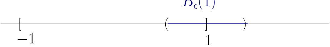
Proof:
Intuitively, any \(\epsilon\)-ball centered on \(1\) will contain points \(> 1\)
More formally, pick any \(\epsilon > 0\) and consider \(B_\epsilon(1)\)
There exists a \(y \in B_\epsilon(1)\) such that \(y \notin [-1, 1]\)
For example, consider the point \(y := 1 + \epsilon/2\)
Exercise: Check this point: lies in \(B_\epsilon(1)\) but not in \([-1, 1]\)
Definition
A set \(G\subset \mathbb{R}^N\) is called open if all of its points are interior
Example
Open sets:
any open interval \((a,b) \subset \mathbb{R}\), since we showed all points are interior
any open ball \(B_\epsilon(a) = x \in \mathbb{R}^N : \|x - a \| < \epsilon\)
\(\mathbb{R}^N\) itself satisfies the defintion of open set
Sets that are not open
\((a,b]\) because \(b\) is not interior
\([a,b)\) because \(a\) is not interior
Closed Sets#
Definition
A set \(F \subset \mathbb{R}^N\) is called closed if every convergent sequence in \(F\) converges to a point in \(F\)
Rephrased: If \(\{x_n\} \subset F\) and \(x_n \to x\) for some \(x \in \mathbb{R}^N\), then \(x \in F\)
Example
All of \(\mathbb{R}^N\) is closed \(\Leftarrow\) every sequence converging to a point in \(\mathbb{R}^N\) converges to a point in \(\mathbb{R}^N\)!
Note that \(\mathbb{R}\) is both open and closed 😲 The empty set \(\varnothing\) is the only other example
Example
If \((-1, 1) \subset \mathbb{R}\) is not closed
Proof:
True because
\(x_n := 1-1/n\) is a sequence in \((-1, 1)\) converging to \(1\),
and yet \(1 \notin (-1, 1)\)
Example
If \(F = [a, b] \subset \mathbb{R}\) then \(F\) is closed in \(\mathbb{R}\)
Proof:
Take any sequence \(\{x_n\}\) such that
\(x_n \in F\) for all \(n\)
\(x_n \to x\) for some \(x \in \mathbb{R}\)
We claim that \(x \in F\)
Recall that (weak) inequalities are preserved under limits:
\(x_n \leq b\) for all \(n\) and \(x_n \to x\), so \(x \leq b\)
\(x_n \geq a\) for all \(n\) and \(x_n \to x\), so \(x \geq a\)
therefore \(x \in [a, b] =: F\)
Properties of Open and Closed Sets#
Fact
\(G \subset \mathbb{R}^N\) is open \(\iff \; G^c\) is closed
Proof
\(\implies\)
First prove necessity
Pick any \(G\) and let \(F := G^c\)
Suppose to the contrary that \(G\) is open but \(F\) is not closed, so
\(\exists\) a sequence \(\{x_n\} \subset F\) with limit \(x \notin F\)
Then \(x \in G\), and since \(G\) open, \(\exists \, \epsilon > 0\) such that \(B_\epsilon(x) \subset G\)
Since \(x_n \to x\) we can choose an \(N \in \mathbb{N}\) with \(x_N \in B_\epsilon(x)\)
This contradicts \(x_n \in F\) for all \(n\)
\(\Longleftarrow\)
Next prove sufficiency
Pick any closed \(F\) and let \(G := F^c\), need to prove that \(G\) is open
Suppose to the contrary that \(G\) is not open
Then exists some non-interior \(x \in G\), that is no \(\epsilon\)-ball around \(x\) lies entirely in \(G\)
Then it is possible to find a sequence \(\{x_n\}\) which converges to \(x \in G\), but every element of which lies in the \(B_{1/n}(x) \cap F\)
This contradicts the fact that \(F\) is closed
Fact
Any singleton \(\{ x \} \subset \mathbb{R}^N\) is closed
Proof
Let’s prove this by showing that \(\{x\}^c\) is open
Pick any \(y \in \{x\}^c\)
We claim that \(y\) is interior to \(\{x\}^c\)
Since \(y \in \{x\}^c\) it must be that \(y \ne x\)
Therefore, exists \(\epsilon > 0\) such that \(B_\epsilon(y) \cap B_\epsilon(x) = \varnothing\)
In particular, \(x \notin B_\epsilon(y)\), and hence \(B_\epsilon(y) \subset \{x\}^c\)
Therefore \(y\) is interior as claimed
Since \(y\) was arbitrary it follows that \(\{x\}^c\) is open and \(\{x\}\) is closed
Fact
Any finite union of open sets is open
Any finite intersection of closed sets is closed
Proof
Proof of first fact:
Let \(G := \cup_{\lambda \in \Lambda} G_\lambda\), where each \(G_\lambda\) is open
We claim that any given \(x \in G\) is interior to \(G\)
Pick any \(x \in G\)
By definition, \(x \in G_\lambda\) for some \(\lambda\)
Since \(G_\lambda\) is open, \(\exists \, \epsilon > 0\) such that \(B_\epsilon(x) \subset G_\lambda\)
But \(G_\lambda \subset G\), so \(B_\epsilon(x) \subset G\) also holds
In other words, \(x\) is interior to \(G\)
But be careful:
An infinite intersection of open sets is not necessarily open
An infinite union of closed sets is not necessarily closed
For example, if \(G_n := (-1/n, 1/n)\), then \(\cap_{n \in \mathbb{N}} G_n = \{0\} \)
Now a very important definition:
Definition
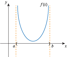
Set \(X\) is called compact if it is both closed and bounded.
Example
Any closed interval \([a, b]\) is a compact
Any hypercube \([a_1, b_1] \times \ldots \times [a_N, b_N]\) is compact
Example
Closed but not compact set is for example
Suprema and Infima (\(\mathrm{sup}\) + \(\mathrm{inf}\))#
Always well defined
Agree with max and min when the latter exist
Definition
Let \(A \subset \mathbb{R}\) (we restrict attention to subsets of real line for now)
A number \(u \in \mathbb{R}\) is called an upper bound of \(A\) if
Example
If \(A = (0, 1)\) then 10 is an upper bound of \(A\) — indeed, every element of \((0, 1)\) is \(\leqslant 10\)
If \(A = (0, 1)\) then 1 is an upper bound of \(A\) — indeed, every element of \((0, 1)\) is \(\leqslant 1\)
If \(A = (0, 1)\) then \(0.75\) is not an upper bound of \(A\)
Definition
Let \(U(A)\) denote set of all upper bounds of \(A\).
A set \(A \subset \mathbb{R}\) is called bounded above if \(U(A)\) is not empty
Examples
If \(A = [0, 1]\), then \(U(A) = [1, \infty)\)
If \(A = (0, 1)\), then \(U(A) = [1, \infty)\)
If \(A = (0, 1) \cup (2, 3)\), then \(U(A) = [3, \infty)\)
If \(A = \mathbb{N}\), then \(U(A) = \varnothing\)
Definition
The least upper bound \(s\) of \(A\) is called supremum of \(A\), denoted \(s=\sup A\), i.e.
Example
If \(A = (0, 1]\), then \(U(A) = [1, \infty)\), so \(\sup A = 1\)
If \(A = (0, 1)\), then \(U(A) = [1, \infty)\), so \(\sup A = 1\)
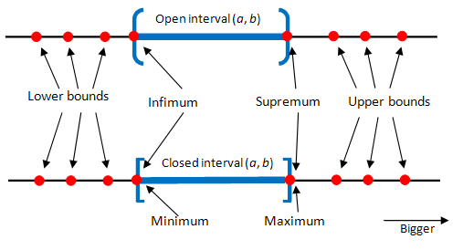
Fig. 27 Upper and lower bounds, supremum and infimum of an interval on \(\mathbb{R}\)#
Definition
A lower bound of \(A \subset \mathbb{R}\) is any \(\ell \in \mathbb{R}\) such that \(\ell \leqslant a\) for all \(a \in A\).
Let \(L(A)\) denote set of all lower bounds of \(A\).
A set \(A \subset \mathbb{R}\) is called bounded below if \(L(A)\) is not empty.
The highest of the lower bounds \(p\) is called the infimum of \(A\), denoted \(p=\inf A\), i.e.
Example
If \(A = [0, 1]\), then \(\inf A = 0\)
If \(A = (0, 1)\), then \(\inf A = 0\)
Some useful facts#
Fact
Boundedness of a subset of the set of real numbers is equivalent to it being bounded above and below.
Proof
The proof follows trivially from the definitions
Fact
Every nonempty subset of \(\mathbb{R}\) bounded above has a supremum in \(\mathbb{R}\)
Every nonempty subset of \(\mathbb{R}\) bounded below has an infimum in \(\mathbb{R}\)
Proof
Similar to the proof that all Cauchy sequences converge, follows from the density property of \(\mathbb{R}\)
Some textbooks allow all sets to have a supremum and infimum, even if they are not bounded. This is achieved by extending the set of real numbers with \(\{-\infty,\infty\}\)
Then, if \(A\) is unbounded above then \(\sup A = \infty\), and if \(A\) is unbounded below then \(\inf A = -\infty\).
Note aside
Conventions for dealing with symbols “\(\infty\)’’ and “\(-\infty\)” If \(a \in \mathbb{R}\), then
\(a + \infty = \infty\)
\(a - \infty = -\infty\)
\(a \times \infty = \infty\) if \(a \ne 0\), \(0 \times \infty = 0\)
\(-\infty < a < \infty\)
\(\infty + \infty = \infty\)
\(-\infty - \infty = -\infty\) But \(\infty - \infty\) is not defined
Fact
Let \(A\) be any set bounded above and let \(s = \sup A\). There exists a sequence \(\{x_n\}\) in \(A\) with \(x_n \to s\).
Analogously, if \(A\) is bounded below and \(p = \inf A\), then there exists a sequence \(\{x_n\}\) in \(A\) with \(x_n \to p\).
Proof
Note that
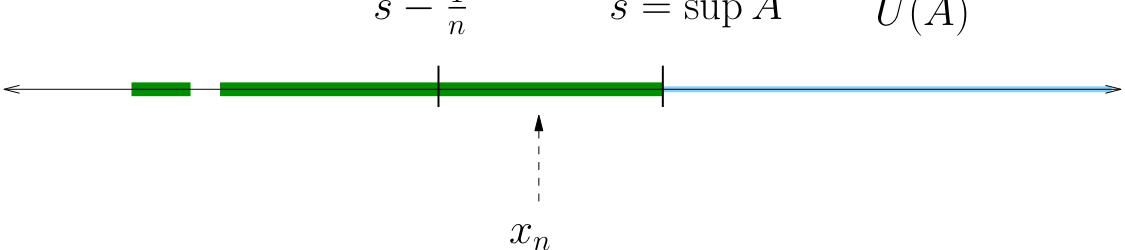
(Otherwise \(s\) is not a sup, because \(s-\frac{1}{n}\) is a smaller upper bound)
The sequence \(\{x_n\}\) lies in \(A\) and converges to \(s\).
The proof for the infimum is analogous.
Maxima and Minima (\(\max\) + \(\min\))#
Definition
We call \(a^*\) the maximum of \(A \subset \mathbb{R}\), denoted \(a^* = \max A\), if
We call \(a^*\) the minimum of \(A \subset \mathbb{R}\) and write \(a^* = \min A\) if
Example
For \(A = [0, 1]\) \(\max A = 1\) and \(\min A = 0\)
Relationship between max/min and sup/inf#
Fact
Let \(A\) be any subset of \(\mathbb{R}\)
If \(\sup A \in A\), then \(\max A\) exists and \(\max A = \sup A\)
If \(\inf A \in A\), then \(\min A\) exists and \(\min A = \inf A\)
In other words, when max and min exist they agree with sup and inf
Proof
Proof of case 1: Let \(a^* = \sup A\) and suppose \(a^* \in A\)
We want to show that \(\max A = a^*\)
Since \(a^* \in A\), we need only show that \(a \leqslant a^*\) for all \(a \in A\)
This follows from \(a^* = \sup A\), which implies \(a^* \in U(A)\)
Fact
If \(F \subset \mathbb{R}\) is a closed and bounded, then \(\max F\) and \(\min F\) both exist
Proof
Proof for the max case:
Since \(F\) is bounded,
\(\sup F\) exists
\(\exists\) a sequence \(\{x_n\} \subset F\) with \(x_n \to \sup F\)
Since \(F\) is closed, this implies that \(\sup F \in F\)
Hence \(\max F\) exists and \(\max F = \sup F\)
Segway to functions#
Of course, in optimization we are mainly interested in maximizing and minimizing functions
Will apply the notions of supremum and infimum, minimum and maximum to the range of a function
Equivalently, we may consider the image of a set \(X \subset \mathbb{R}^N\) under a function \(f\)
Definition
Let \(f \colon A \to \mathbb{R}\), where \(A\) is any set
The supremum of \(f\) on \(A\) is defined as
The infimum of \(f\) on \(A\) is defined as
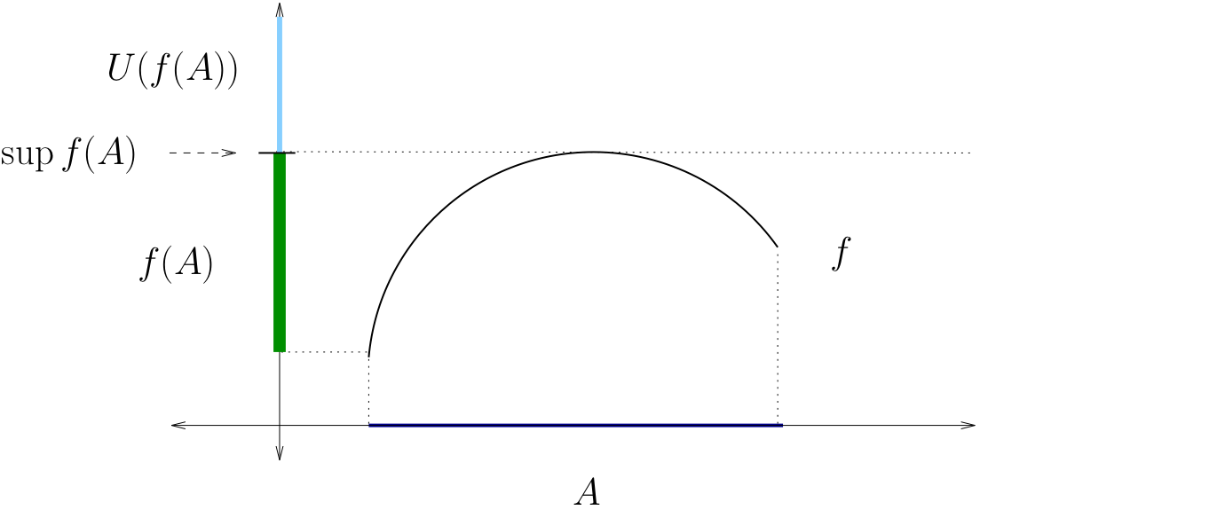
Fig. 28 The supremum of \(f\) on \(A\)#
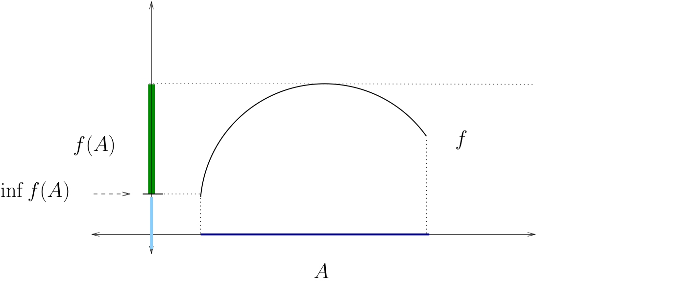
Fig. 29 The infimum of \(f\) on \(A\)#
Definition
Let \(f \colon A \to \mathbb{R}\) where \(A\) is any set
The maximum of \(f\) on \(A\) is defined as
The minimum of \(f\) on \(A\) is defined as
Definition
A maximizer of \(f\) on \(A\) is a point \(a^* \in A\) such that
The set of all maximizers is typically denoted by
Definition
A minimizer of \(f\) on \(A\) is a point \(a^* \in A\) such that
The set of all minimizers is typically denoted by
Weierstrass boundedness theorem#
Putting together all the above material to formulate a fundamental result which is essential for establishing the existence of maxima and minima of functions in the next section.
Definition
A function \(f\) is called bounded if its range is a bounded set.
Example
\([0,1] \ni x \mapsto f(x) = x^5 \in \mathbb{R}\) is bounded
\(\sin(x)\) is bounded on \(\mathbb{R}\), i.e. \(f: \mathbb{R} \to \mathbb{R}\) where \(f(x) = \sin(x)\) is bounded
\(f(x)=1/x\) is not bounded (on \(\mathbb{R}\))
\(f(x) = \log(x)\) is not bounded (on \(\mathbb{R}\))
Fact
Consider a continuous function \(f: X \subset \mathbb{R}^N \to \mathbb{R}\).
If \(X\) is compact, then \(f\) is bounded on \(X\).
Proof
Sketch of the proof:
Suppose that range of \(f\) denoted \(f(X)\) is not a bounded set
Then we can find a sequence \(\{x_n\}\) in \(X\) such that \(\forall n\in\mathbb{N}\) \(f(x_n)\) such that \(|f(x_n)|>n\), i.e. the sequence \(\{f(x_n)\}\) is unbounded.
Sequence \(\{x_n\}\) is bounded, so by Bolzano-Weierstrass theorem it has a convergent subsequence \(\{x_{n_k}\}\), where \(n_k\) is a subset of \(\mathbb{N}\) index by \(k\), and thus \(k \leqslant n_k\) for all \(k\)
Denote by \(L\) the limit of this subsequence, \(L = \lim_{k \to \infty} \{x_{n_k}\}\)
\(L \in X\) because \(X\) is a compact and thus is a closed set
By continuity of \(f\) at \(L\) we have that \(f(x_{n_k}) \to f(L)\)
Then the sequence \(\{f(x_{n_k})\}\) is bounded due to the properties of the limit, see relevant fact
However, by construction \(|f(x_{n_k})| > n_k \geqslant k\) where \(k\) can be arbitrary large
We have a contradiction, therefore the range of \(f\) must be bounded
Also see the discussion here
Weierstrass extreme value theorem#
Fundamental result on existence of maxima and minima of functions!
Classic example of an existance theorem: it states that something exists without providing a method to find it
Fact (Weierstrass extreme value theorem)
If \(f: A \subset \mathbb{R}^N \to \mathbb{R}\)
is continuous and \(A\) is closed and bounded (compact),
then \(f\) has both a maximizer and a minimizer on \(A\).
Proof
Sketch of the proof:
If \(f\) is continuous and \(A\) is compact, then \(f(A)\) is bounded, see relevant fact
Because \(f(A)\) is bounded \(\sup f(A)\) and \(\inf f(A)\) exist, see relevant fact
There is a sequence \(\{y_n\} \in f(A)\) converging to sup/inf, see relevant fact
Consider the corresponding sequence of \(\{x_n\}\) such that \(y_n=f(x_n)\)
It may not be convergent, but is bounded (belongs to compact), therefore contains a convergent subsequence \(\{x_{n_k}\}\) (by Bolzano-Weierstrass theorem), see relevant fact
Let \(c\) be the limit of a convergent subsequence: \(x_{n_k} \to c\) as \(k \to \infty\)
Then by definition of continuity \(f(c)\) is the limit of the sequence \(f(x_{n_k})\)
\(f(c)\) must then be the same as the limit of the sequence \(y_n\) = sup/inf due to the fact that any sequence can have at most one limit, see relevant fact
Therefore sup/inf is attained at \(x=c\)
Becasue \(c\) is in \(A\), \(f(c)\) is in the range of \(f\), and thus \(f\) sup/inf can be replaced by max/min, see relevant fact
Therefore \(c\) is a maximizer/minimizer
Example
Consider the problem
where
\(r \in (0,1)\) is interest rate
\(w\) is wealth
\(\beta \in (0,1)\) is a discount factor
Let \(B\) be all \((c_1, c_2)\) satisfying the constraint
Exercise: Show that the budget set \(B\) is a closed, bounded subset of \(\mathbb{R}^2\)
Exercise: Show that \(U\) is continuous on \(B\)
We conclude that a maximizer exists
Example
Examples of failure of Weierstrass theorem conditoins
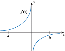
Why? Function is not continuous on \([a,b]\)
Why? Domain of the function is not closed
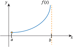
Why? The function is not continuous or not defined at the right endpoint of the interval: either continuity or closedness is violated