📖 Constrained optimization#
⏱ | words
References and additional materials
Setting up a constrained optimization problem#
Let’s start with recalling the definition of a general optimization problem
Definition
The general form of the optimization problem is
where:
\(f(x,\theta) \colon \mathbb{R}^N \times \mathbb{R}^K \to \mathbb{R}\) is an objective function
\(x \in \mathbb{R}^N\) are decision/choice variables
\(\theta \in \mathbb{R}^K\) are parameters
\(g_i(x,\theta) = 0, \; i\in\{1,\dots,I\}\) where \(g_i \colon \mathbb{R}^N \times \mathbb{R}^K \to \mathbb{R}\), are equality constraints
\(h_j(x,\theta) \le 0, \; j\in\{1,\dots,J\}\) where \(h_j \colon \mathbb{R}^N \times \mathbb{R}^K \to \mathbb{R}\), are inequality constraints
\(V(\theta) \colon \mathbb{R}^K \to \mathbb{R}\) is a value function
Today we focus on the problem with constrants, i.e. \(I+J>0\)
The obvious classification that we follow
equality constrained problems, i.e. \(I>0\), \(J=0\)
inequality constrained problems, i.e. \(J>0\), which can include equalities as special case
Note
Note that every optimization problem can be seen as constrained if we define the objective function to have the domain that coincides with the admissible set.
is equivalent to
Constrained Optimization = economics#
A major focus of econ: the optimal allocation of scarce resources
optimal = optimization
scarce = constrained
Standard constrained problems:
Maximize utility given budget
Maximize portfolio return given risk constraints
Minimize cost given output requirement
Example
Maximization of utility subject to budget constraint
\(p_i\) is the price of good \(i\), assumed \(> 0\)
\(m\) is the budget, assumed \(> 0\)
\(x_i \geq 0\) for \(i = 1,2\)
let \(u(x_1, x_2) = \alpha \log(x_1) + \beta \log(x_2)\), \(\alpha>0\), \(\beta>0\)
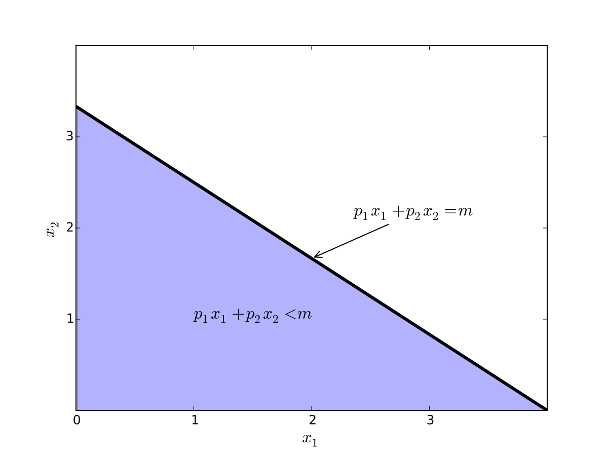
Fig. 63 Budget set when, \(p_1=0.8\), \(p_2 = 1.2\), \(m=4\)#
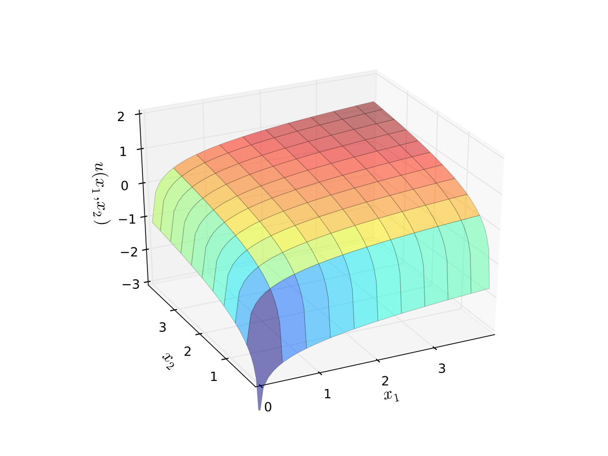
Fig. 64 Log utility with \(\alpha=0.4\), \(\beta=0.5\)#
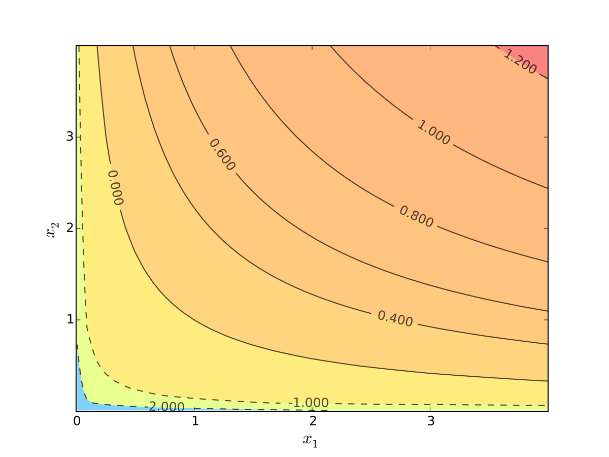
Fig. 65 Log utility with \(\alpha=0.4\), \(\beta=0.5\)#
We seek a bundle \((x_1^\star, x_2^\star)\) that maximizes \(u\) over the budget set
That is,
for all \((x_1, x_2)\) satisfying \(x_i \geq 0\) for each \(i\) and
Visually, here is the budget set and objective function:
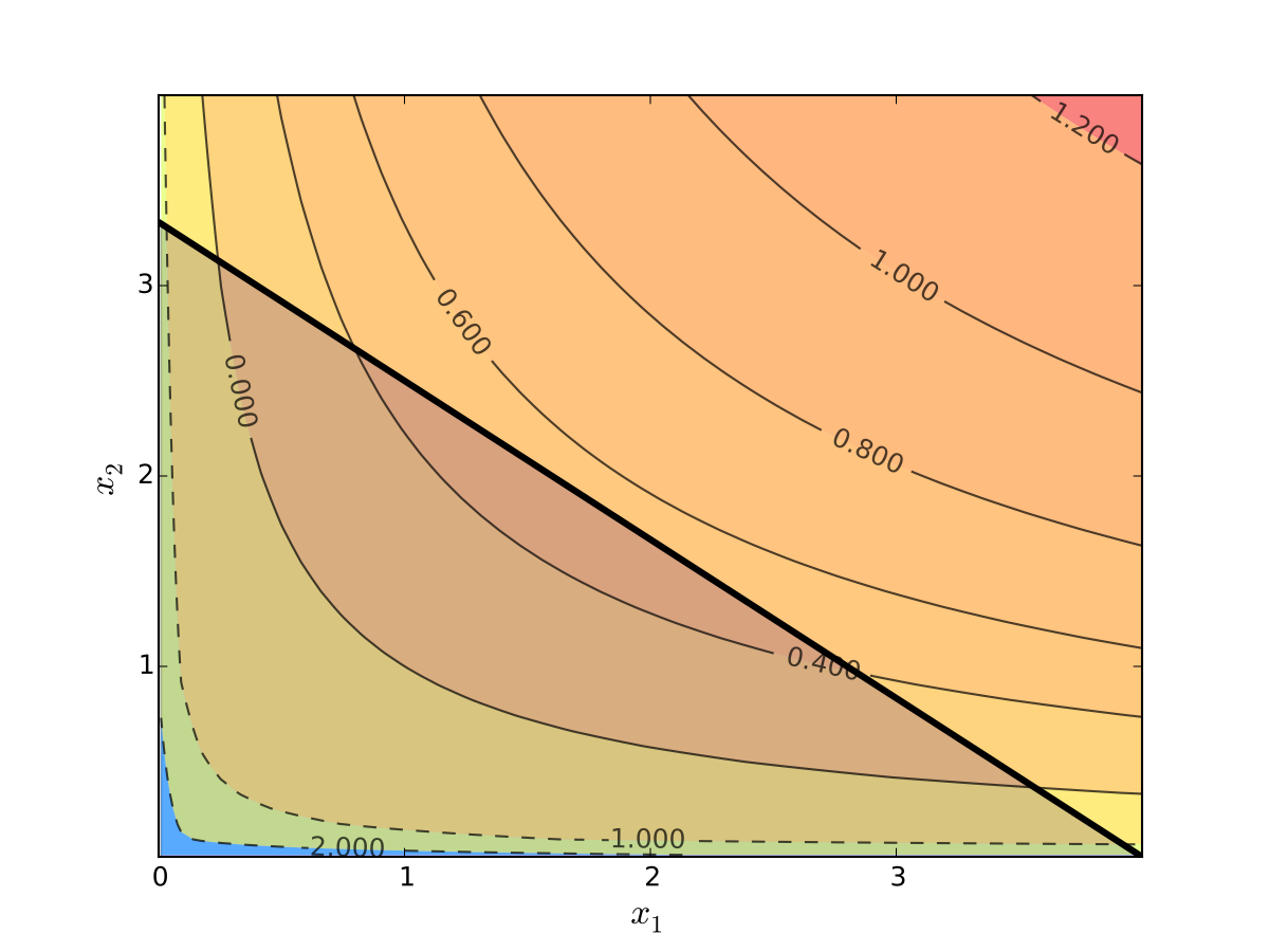
Fig. 66 Utility max for \(p_1=1\), \(p_2 = 1.2\), \(m=4\), \(\alpha=0.4\), \(\beta=0.5\)#
First observation: \(u(0, x_2) = u(x_1, 0) = u(0, 0) = -\infty\)
Hence we need consider only strictly positive bundles
Second observation: \(u(x_1, x_2)\) is strictly increasing in both \(x_i\)
Never choose a point \((x_1, x_2)\) with \(p_1 x_1 + p_2 x_2 < m\)
Otherwise can increase \(u(x_1, x_2)\) by small change
Hence we can replace \(\leq\) with \(=\) in the constraint
Implication: Just search along the budget line
Substitution Method#
Substitute constraint into objective function and treat the problem as unconstrained
This changes
into
Since all candidates satisfy \(x_1 > 0\) and \(x_2 > 0\), the domain is
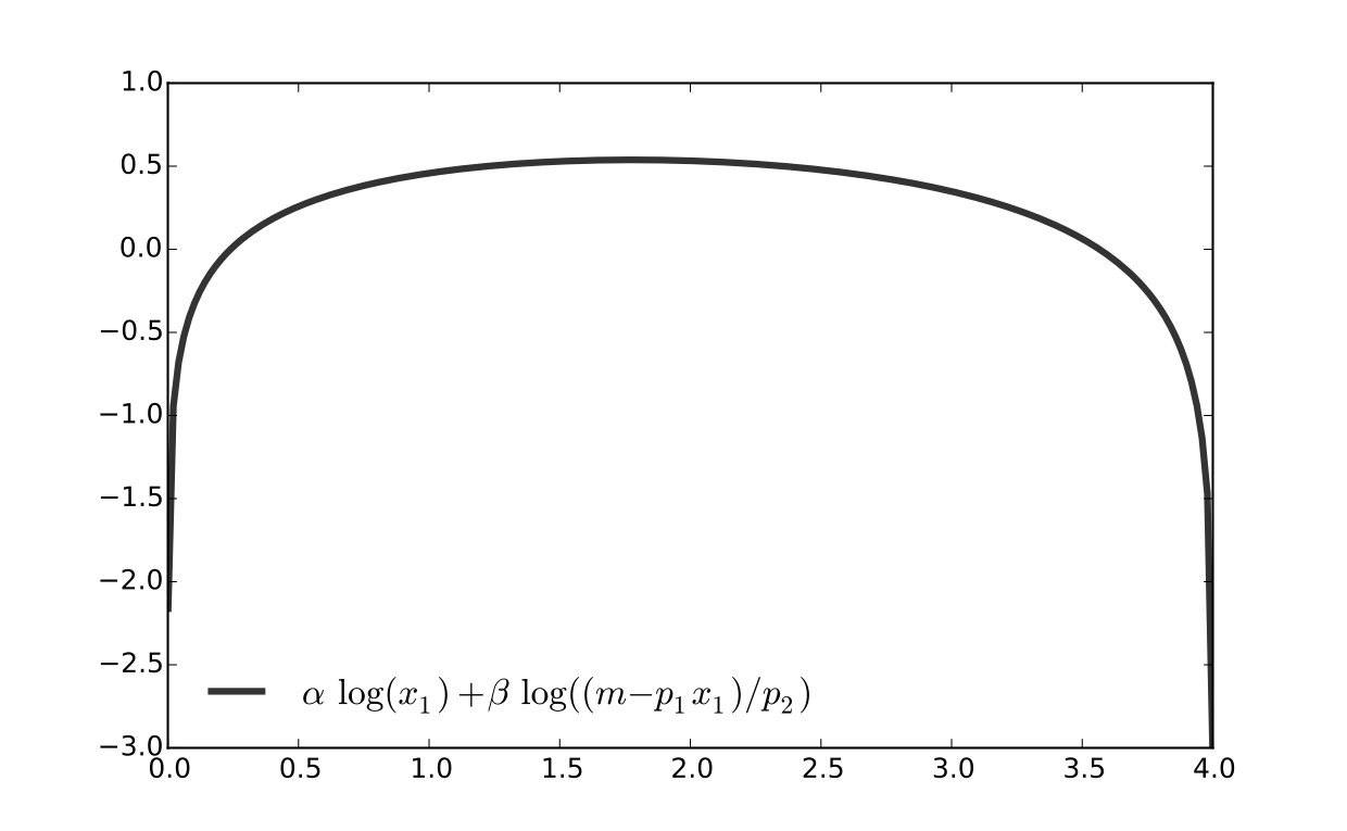
Fig. 67 Utility max for \(p_1=1\), \(p_2 = 1.2\), \(m=4\), \(\alpha=0.4\), \(\beta=0.5\)#
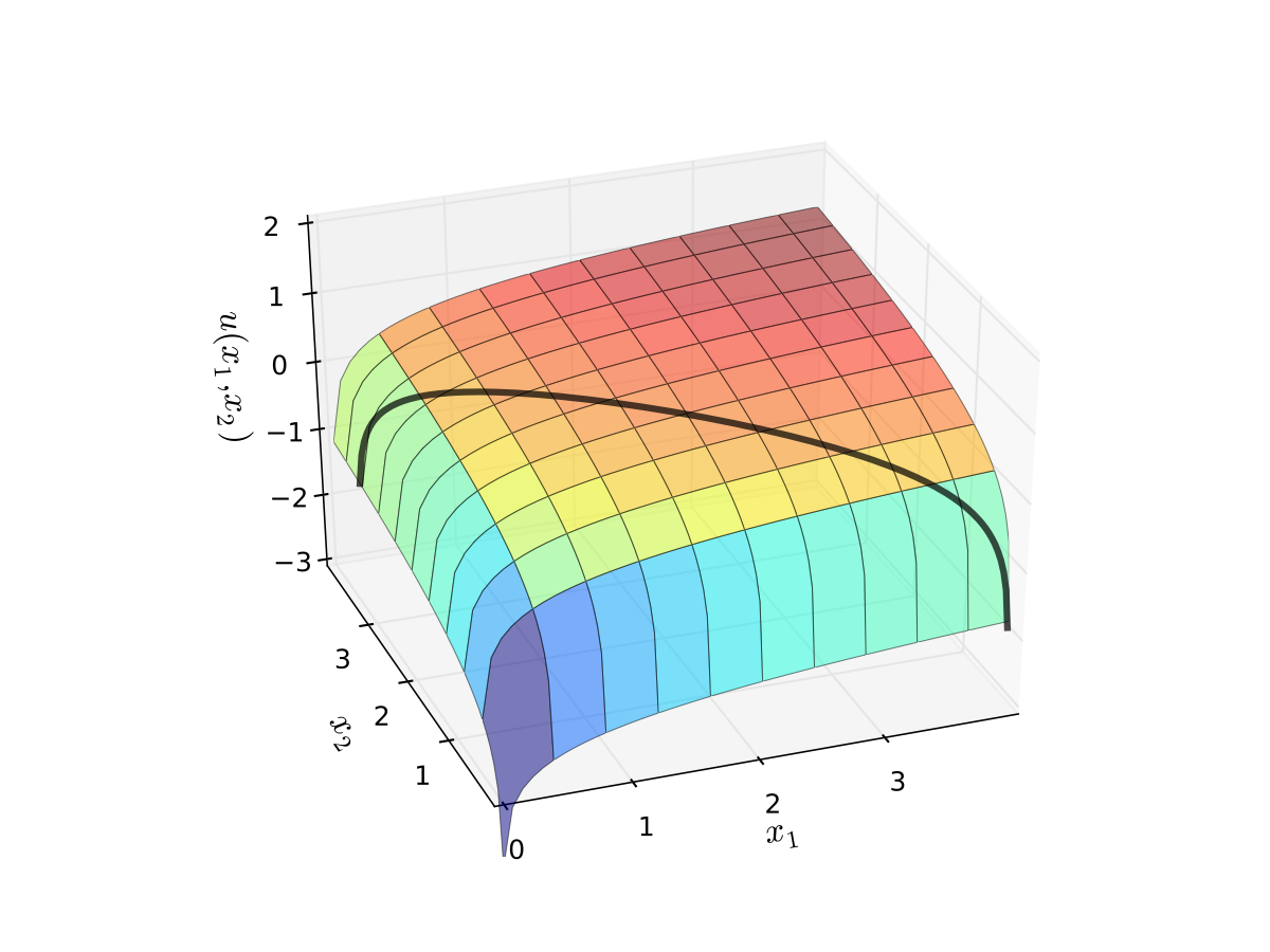
Fig. 68 Utility max for \(p_1=1\), \(p_2 = 1.2\), \(m=4\), \(\alpha=0.4\), \(\beta=0.5\)#
First order condition for
gives
Exercise: Verify
Exercise: Check second order condition (strict concavity)
Substituting into \(p_1 x_1^\star + p_2 x_2^\star = m\) gives
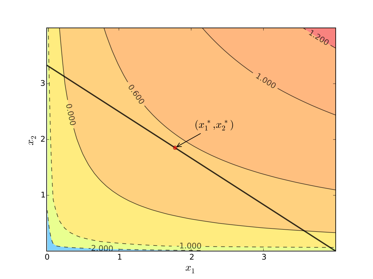
Fig. 69 Maximizer for \(p_1=1\), \(p_2 = 1.2\), \(m=4\), \(\alpha=0.4\), \(\beta=0.5\)#
Substitution method: algorithm#
How to solve
Steps:
Write constraint as \(x_2 = h(x_1)\) for some function \(h\)
Solve univariate problem \(\max_{x_1} f(x_1, h(x_1))\) to get \(x_1^\star\)
Plug \(x_1^\star\) into \(x_2 = h(x_1)\) to get \(x_2^\star\)
Limitations: substitution doesn’t always work
Example
Suppose that \(g(x_1, x_2) = x_1^2 + x_2^2 - 1\)
Step 1 from the cookbook says
use \(g(x_1, x_2) = 0\) to write \(x_2\) as a function of \(x_1\)
But \(x_2\) has two possible values for each \(x_1 \in (-1, 1)\)
In other words, \(x_2\) is not a well defined function of \(x_1\)
As we meet more complicated constraints such problems intensify
Constraint defines complex curve in \((x_1, x_2)\) space
Inequality constraints, etc.
We need more general, systematic approach
Tangency and relative slope conditions#
Optimization approach based on tangency of contours and constraints
Example
Consider again the problem
Turns out that the maximizer has the following property:
budget line is tangent to an indifference curve at maximizer
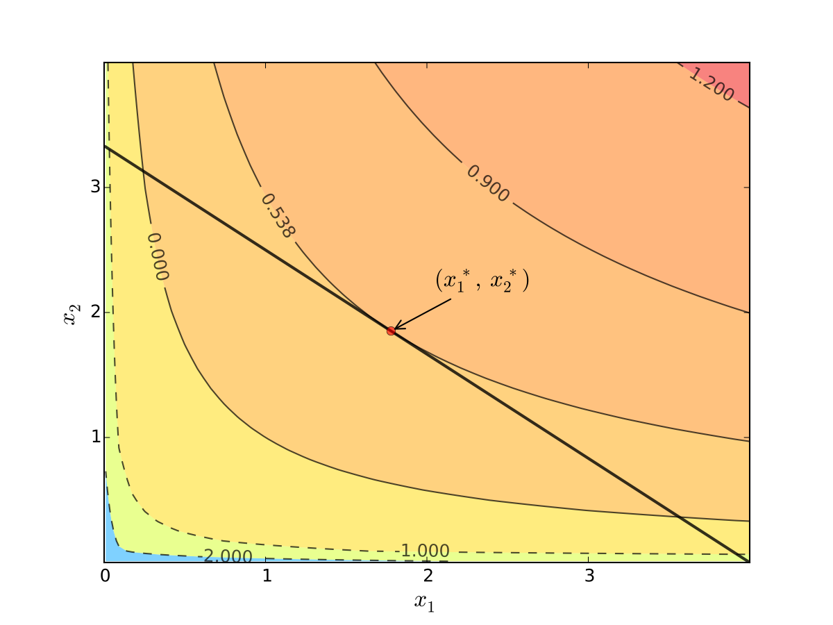
Fig. 70 Maximizer for \(p_1=1\), \(p_2 = 1.2\), \(m=4\), \(\alpha=0.4\), \(\beta=0.5\)#
In fact this is an instance of a general pattern
Notation: Let’s call \((x_1, x_2)\) interior to the budget line if \(x_i > 0\) for \(i=1,2\) (not a “corner” solution, see below)
In general, any interior maximizer \((x_1^\star, x_2^\star)\) of differentiable utility function \(u\) has the property: budget line is tangent to a contour line at \((x_1^\star, x_2^\star)\)
Otherwise we can do better:
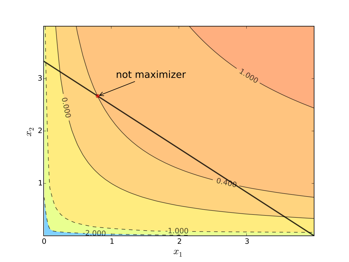
Fig. 71 When tangency fails we can do better#
Necessity of tangency often rules out a lot of points
We exploit this fact to build intuition and develop more general method
Relative Slope Conditions#
Consider an equality constrained optimization problem where objective and constraint functions are differentiable:
How to develop necessary conditions for optima via tangency?
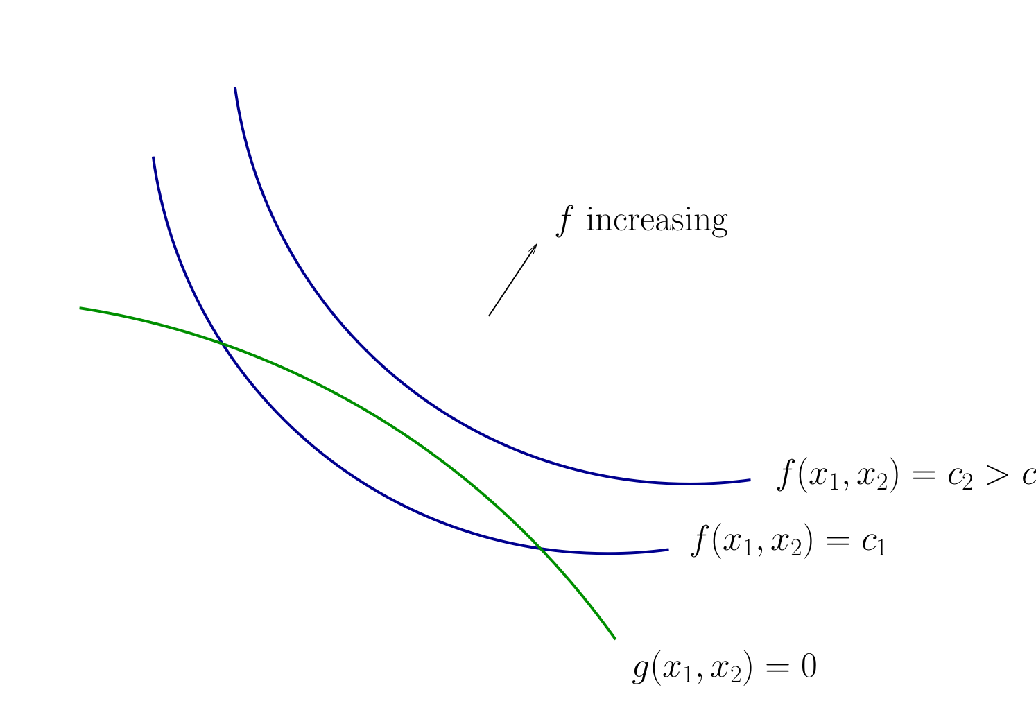
Fig. 72 Contours for \(f\) and \(g\)#
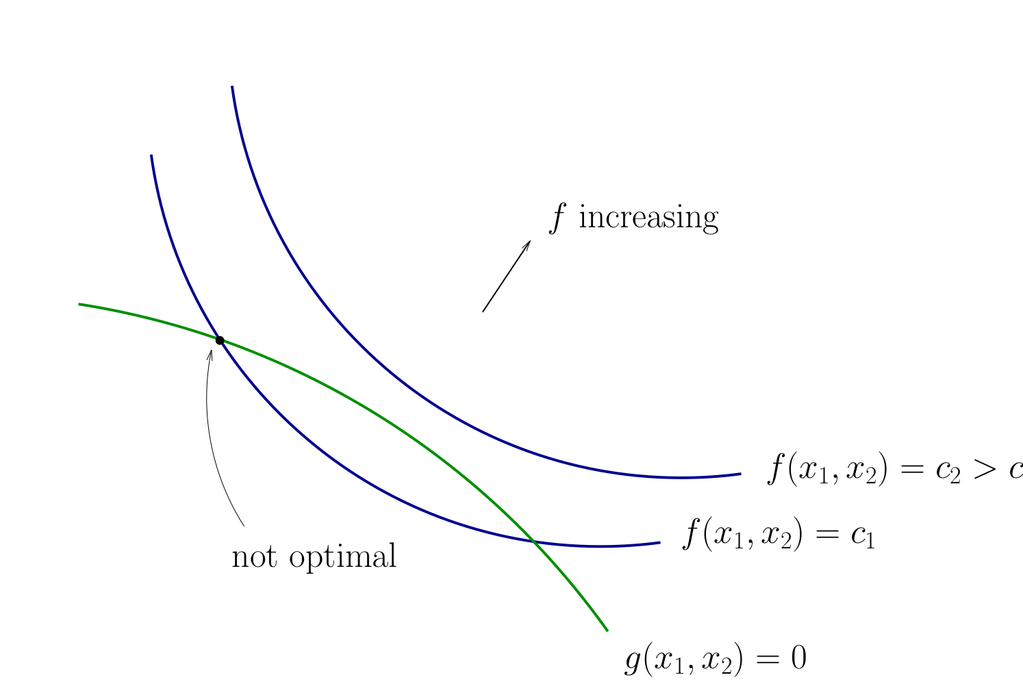
Fig. 73 Contours for \(f\) and \(g\)#
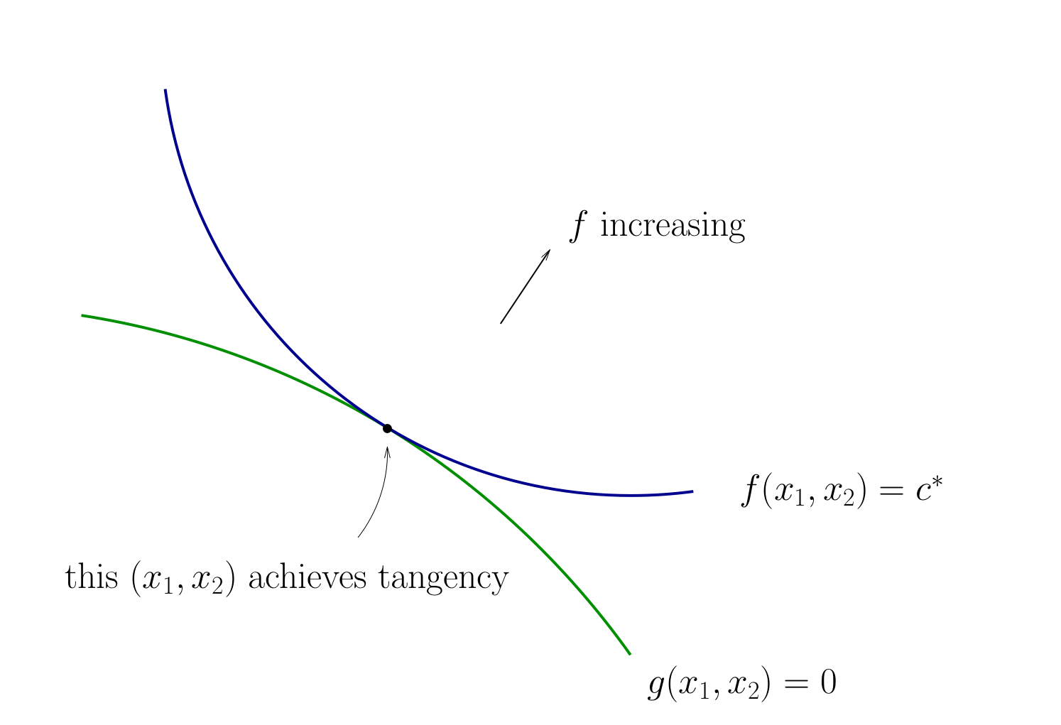
Fig. 74 Tangency necessary for optimality#
How do we locate an optimal \((x_1, x_2)\) pair?
Diversion: derivative of an implicit function
To continue with the tangency approach we need to know how to differentiate an implicit function \(x_2(x_1)\) which is given by a contour line of the utility function \(f(x_1, x_2)=c\)
Let’s approach this task in the following way
utility function is given by \(f \colon \mathbb{R}^2 \to \mathbb{R}\)
the contour line is given by \(f(x_1,x_2) = c\) which defines an implicit function \(x_1(x_2)\)
let map \(g \colon \mathbb{R} \to \mathbb{R}^2\) given by \(g(x_2) = \big[x_1(x_2),x_2\big]\)
The total derivative matrix of \(f \circ g\) can be derived using the chain rule
Differentiating the equation \(f(x_1,x_2) = c\) on both sides with respect to \(x_2\) gives \(D(f \circ g)(x) = 0\), thus leading to the final expression for the derivative of the implicit function
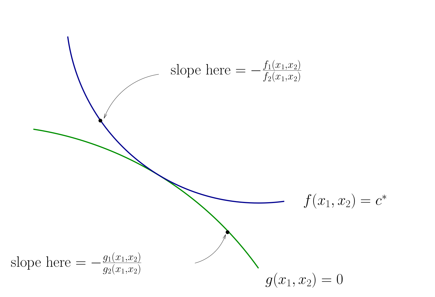
Fig. 75 Slope of contour lines#
Let’s choose \((x_1, x_2)\) to equalize the slopes
That is, choose \((x_1, x_2)\) to solve
Equivalent:
Also need to respect \(g(x_1, x_2) = 0\)
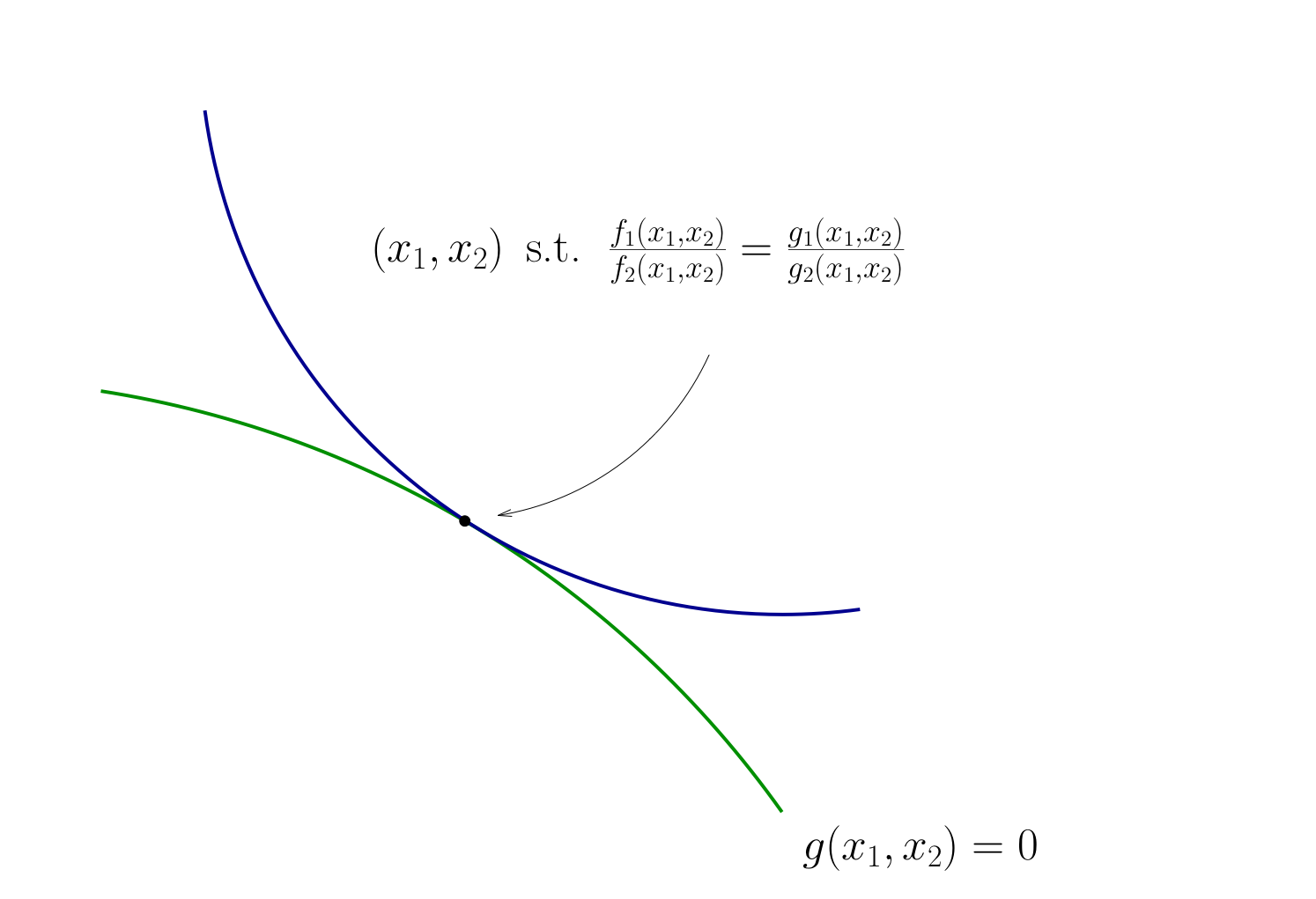
Fig. 76 Condition for tangency#
Tangency condition algorithm#
In summary, when \(f\) and \(g\) are both differentiable functions, to find candidates for optima in
(Impose slope tangency) Set
(Impose constraint) Set \(g(x_1, x_2) = 0\)
Solve simultaneously for \((x_1, x_2)\) pairs satisfying these conditions
Example
Consider again
Then
Solving simultaneously with \(p_1 x_1 + p_2 x_2 = m\) gives
Same as before…
This approach can be applied to maximization as well as minimization problems
Note
The methods described here
substitution method
tangency/relative slope method
are applicable to simple constrained optimization problems with intuitive constraints
But what about more complicated problems? Necessary and sufficient first order conditions? Second order conditions?
We need more general approach for that \(\longrightarrow\) the method of Lagrange multipliers