📖 Envelope theorem

Issues with the online test 4 😬
- questions on the Envelope theorem were included by mistake
- marks for these questions will be set to full mark
- if you had such question, the grade will be adjusted
- manual adjustments are needed, so be patient
Don’t forget the deadline of May 23 for the individual project
- Let me know if you have any questions or concerns

📖 Envelope theorem#

⏱ | words

Value function with parameters#

Let’s start with recalling the definition of a general optimization problem

Definition

The general form of the optimization problem is

\[\begin{split} V(\theta) = \max_{x} f(x,\theta) \\ \text {subject to} \\ g_i(x,\theta) = 0, \; i\in\{1,\dots,I\}\\ h_j(x,\theta) \le 0, \; j\in\{1,\dots,J\} \end{split}\]

where:

\(f(x,\theta) \colon \mathbb{R}^N \times \mathbb{R}^K \to \mathbb{R}\) is an objective function
\(x \in \mathbb{R}^N\) are decision/choice variables
\(\theta \in \mathbb{R}^K\) are parameters
\(g_i(x,\theta) = 0, \; i\in\{1,\dots,I\}\) where \(g_i \colon \mathbb{R}^N \times \mathbb{R}^K \to \mathbb{R}\), are equality constraints
\(h_j(x,\theta) \le 0, \; j\in\{1,\dots,J\}\) where \(h_j \colon \mathbb{R}^N \times \mathbb{R}^K \to \mathbb{R}\), are inequality constraints
\(V(\theta) \colon \mathbb{R}^K \to \mathbb{R}\) is a value function

This lecture focuses on the value function in the optimization problem \(V(\theta)\), and how it depends on the parameters \(\theta\).

In economics we are interested how the optimized behavior changes when the circumstances of the decision-making process change

income/budget/wealth changes
intertemporal effects of changes in other time periods

We would like to establish the properties of the value function \(V(\theta)\):

continuity \(\rightarrow\) The maximum theorem (not covered here, see additional lecture notes)
changes/derivative (if differentiable) \(\rightarrow\) Envelope theorem
monotonicity \(\rightarrow\) Supermodularity and increasing differences (not covered here, see Sundaram ch.10)

Unconstrained optimization case#

Let’s start with an unconstrained optimization problem

\[ V(\theta) = \max_{x} f(x,\theta) \]

where:

\(f(x,\theta) \colon \mathbb{R}^N \times \mathbb{R}^K \to \mathbb{R}\) is an objective function
\(x \in \mathbb{R}^N\) are decision/choice variables
\(\theta \in \mathbb{R}^K\) are parameters
\(V(\theta) \colon \mathbb{R}^K \to \mathbb{R}\) is a value function

Envelope theorem for unconstrained problems

Let \(f(x,\theta) \colon \mathbb{R}^N \times \mathbb{R}^K \to \mathbb{R}\) be a differentiable function, and \(x^\star(\theta)\) be the maximizer of \(f(x,\theta)\) for every \(\theta\). Suppose that \(x^\star(\theta)\) is differentiable function itself. Then the value function of the problem \(V(\theta) = f\big(x^\star(\theta),\theta)\) is differentiable w.r.t. \(\theta\) and

\[ \forall j \;\; \frac{\partial V}{\partial \theta_j} = \frac{\partial f}{\partial \theta_j} \big(x^\star(\theta),\theta\big) = \left.\frac{\partial f}{\partial \theta_j} \right|_{x^\star(\theta),\theta} \]

In other words, the marginal changes in the value function are given by the partial derivative of the objective function with respect to the parameter, evaluated at the maximizer.

When \(K=1\), so that \(\theta\) is a scalar, the envelope theorem can be written as

\[ \frac{d V(\theta)}{d \theta} = \frac{d f\big(x^\star(\theta),\theta\big)}{d \theta} = \frac{\partial f\big(x^\star(\theta),\theta\big)}{\partial \theta} = f^\prime_2\big(x^\star(\theta),\theta\big) \]

Note that the total derivative of the objective function at the optimizer is equal to the partial derivative of the objective function with respect to the parameter \(\theta\), evaluated at teh optimizer. The meaning is carried only by the derivative symbol!

Proof

Using the chain rule, we have

\[ \frac{\partial V(\theta)}{\partial \theta_i} = \frac{\partial f\big(x^\star(\theta),\theta\big)}{\partial \theta_i} = \sum_{j=1}^{N} \underbrace{\frac{\partial f\big(x^\star(\theta),\theta\big)}{\partial x_j}}_{=0 \text{ by FOC}} \frac{\partial x_j^\star(\theta)}{\partial \theta_i} + \frac{\partial f\big(x^\star(\theta),\theta\big)}{\partial \theta_i} \]

See also Theorem 19.4 in Simon and Blume (1994), pp. 453-454

Example

Consider \(f(x,a) = -x^2 +2ax +4a^2 \to \max_x\).
What is the (approximate) effect of a unit increase in \(a\) on the attained maximum?

FOC: \(-2x+2a=0\), giving \(x^\star(a) = a\).

So, \(V(a) = f(a,a) = 5a^2\), and \(V'(a)=10a\). The value increases at a rate of \(10a\) per unit increase in \(a\).

Using the envelope theorem, we could go directly to

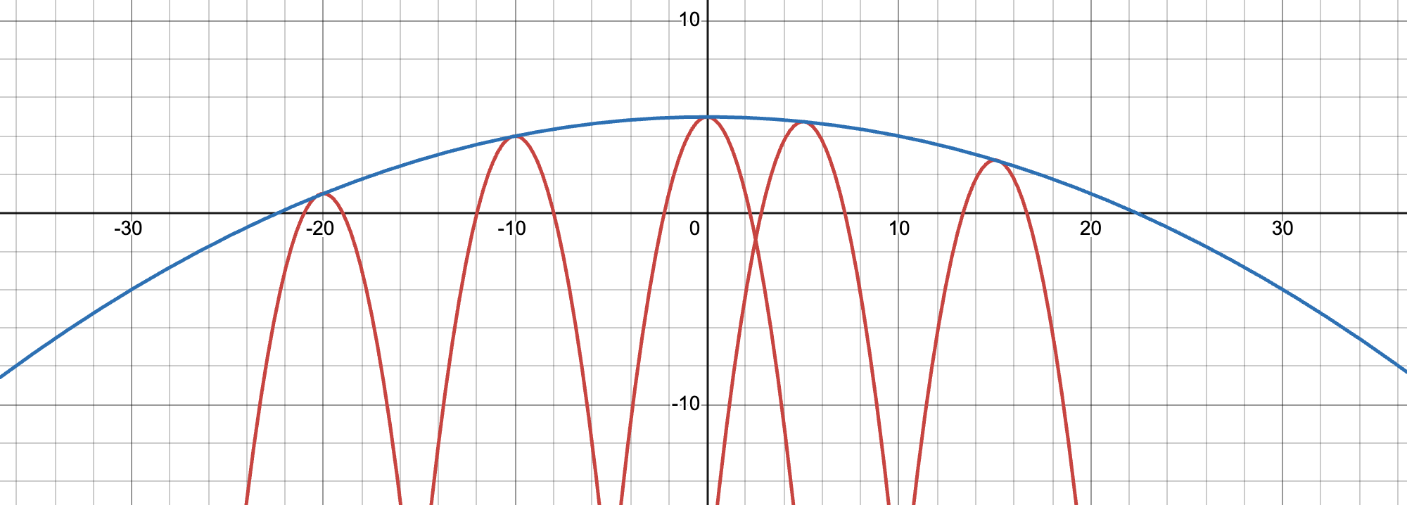
\[ V'(a) = \frac{\partial f}{\partial a} (x^\star(a),a) = 2x + 8a \Big|_{x=a} = 10a \]

Example

\[ f(x,a) = 5 - (x-a)^2 - a^2/100 \to \max_x \]

Clearly \(x^\star(a)=a\). By envelope theorem

\[ \frac{d f(x^\star(a),a)}{d a} = \left.\frac{\partial f}{\partial a}\right|_{x^\star(a)} = \left. 2(x-a)-\frac{a}{50}\right|_{x^\star(a)} = -\frac{a}{50} \]

To make an ``envelope’’ blue line, we can plot \(e(x) = f(x,(x^\star)^{-1}(x)) = 5-x^2/100\)

See live example in Desmos

Constrained optimization case#

Envelope theorem for constrained problems

Consider an equality constrained optimization problem

\[\begin{split} V(\theta) = \max_{x} f(x,\theta) \\ \text {subject to} \\ g_i(x,\theta) = 0, \; i\in\{1,\dots,I\}\\ \end{split}\]

where:

\(f(x,\theta) \colon \mathbb{R}^N \times \mathbb{R}^K \to \mathbb{R}\) is an objective function
\(x \in \mathbb{R}^N\) are decision/choice variables
\(\theta \in \mathbb{R}^K\) are parameters
\(g_i(x,\theta) = 0, \; i\in\{1,\dots,I\}\) where \(g_i \colon \mathbb{R}^N \times \mathbb{R}^K \to \mathbb{R}\), are equality constraints
\(V(\theta) \colon \mathbb{R}^K \to \mathbb{R}\) is a value function

Assume that the maximizer correspondence \(\mathcal{D}^\star(\theta) = \mathrm{arg}\max f(x,\theta)\) is single-valued and can be represented by the function \(x^\star(\theta) \colon \mathbb{R}^K \to \mathbb{R}^N\), with the corresponding Lagrange multipliers \(\lambda^\star(\theta) \colon \mathbb{R}^K \to \mathbb{R}^I\).

Assume that both \(x^\star(\theta)\) and \(\lambda^\star(\theta)\) are differentiable, and that the constraint qualification assumption holds. Then

\[ \frac{\partial V}{\partial \theta_j} = \frac{\partial \mathcal{L}}{\partial \theta_j} \big(x^\star(\theta),\lambda^\star(\theta),\theta\big), \forall j \]

where \(\mathcal{L}(x,\lambda,\theta)\) is the Lagrangian of the problem.

Proof

Here is a version of proof. The Lagrangian is

\[ \mathcal{L}(x^\star(\theta),\lambda^\star(\theta), \theta) = f(x^\star(\theta),\theta)- \sum_{i=1}^{I}\lambda_{i}^\star(\theta) g_{i}(x^\star(\theta), \theta ) \]

Start by exploring its partial derivatives with respect to \(\theta_{j}\), \(j=1,\dots,K\)

\[\begin{split} \frac{\partial\mathcal{L}(x^\star(\theta), \lambda^\star(\theta), \theta)}{\partial{\theta_{j}}} &= \frac{\partial f(x^\star(\theta), \theta)}{\partial{\theta_{j}}} - \sum_{i=1}^{I} \left[ \frac{\partial\lambda_{i}^\star(\theta)}{\partial \theta_{j}}g_{i}(x^\star(\theta), \theta) + \lambda_{i}^\star(\theta) \frac{\partial g_{i}(x^\star(\theta), \theta) }{\partial \theta_{j}}\right] \\ &= \frac{\partial f(x^\star(\theta), \theta)}{\partial{\theta_{j}}} - \sum_{i=1}^{I} \lambda_{i}^\star(\theta) \frac{\partial g_{i}(x^\star(\theta), \theta) }{\partial \theta_{j}} \end{split}\]

We use the fact that the equality constraints \(g_{i}(x^\star(\theta), \theta)=0\) hold for all \(i\).

Now we differentiate the value function w.r.t. \(\theta_{j}\) and show that it is equal to the same expression as above.

\[ \frac{\partial V(\theta)}{\partial{\theta_{j}}} = \frac{d f(x^\star(\theta),\theta)}{d \theta_{j}} = \sum_{n=1}^{N} \frac{\partial f(x^\star(\theta), \theta)}{\partial x_{n}} \frac{\partial x_n(\theta)}{\partial \theta_{j}} +\frac{\partial f(x^\star(\theta), \theta) }{\partial \theta_{j}} = \]

Now we use the fact that first order conditions hold at \((x^\star,\lambda^\star)\) and we have

\[\begin{split} \begin{array}{rl} 0 = \frac{\partial\mathcal{L}(x^\star(\theta), \lambda^\star(\theta), \theta)}{\partial{x_n}} &= \frac{\partial f(x^\star(\theta), \theta)}{\partial{x_n}} - \sum_{i=1}^{I} \lambda_{i}^\star(\theta) \frac{\partial g_{i}(x^\star(\theta), \theta) }{\partial x_{n}}, \\ \end{array} \end{split}\]

Continuing the main line

\[\begin{split} = \sum_{n=1}^{N} \left(\sum_{i=1}^{I}\lambda_{i} \frac{\partial g_i(x^\star(\theta), \theta)}{\partial x_{n}} \right)\frac{\partial x_{n}(\theta)}{ \partial \theta_{j}} +\frac{\partial f(x^\star(\theta), \theta) }{\partial \theta_{j}} =\\= \sum_{i=1}^{I}\lambda_{i} \sum_{n=1}^{N} \frac{\partial g_i(x^\star(\theta), \theta)}{\partial x_{n}}\frac{\partial x_{n}(\theta)}{\partial\theta_{j}} +\frac{\partial f(x^\star(\theta), \theta) }{\partial \theta_{j}} = \end{split}\]

Here we use the fact that the constraints hold, and thus differentiating both side we have

\[\begin{split} \begin{array}{rl} g_{i}(x^\star(\theta), \theta) &=0 \\ \frac{\partial}{\partial \theta_{j}} g_{i}(x^\star(\theta), \theta) &= \frac{\partial}{\partial \theta_{j}} 0 \\ \sum_{n=1}^{N} \frac{\partial g_i(x^\star(\theta), \theta)}{\partial x_{n}}\frac{\partial x_{n}(\theta)}{ \partial\theta_{j}} + \frac{\partial g_i(x^\star(\theta), \theta)}{\partial \theta_{j}} &= 0 \end{array} \end{split}\]

Continuing the main line

\[\begin{split} = - \sum_{i=1}^{I}\lambda_{i} \frac{\partial g_i(x^\star(\theta), \theta)}{\partial \theta_j} +\frac{\partial f(x^\star(\theta), \theta) }{\partial \theta_{j}} =\\= \frac{\partial\mathcal{L}(x^\star(\theta), \lambda^\star(\theta), \theta)}{\partial{\theta_{j}}} \end{split}\]

\(\blacksquare\)

Note

What about the inequality constraints?

Well, if the solution is interior and none of the constrains are binding, the unconstrained version of the envelope theorem applies. If any of the constrains are binding, their combination can be represented as a set of equality constraint, and the constrained version of the envelope theorem applies. Care needs to be taken to avoid the changes in the parameter that lead to a switch in the binding constraints. Such points are most likely non-differentiable, and the envelope theorem does not apply there at all!

Example

Back to the log utility case

\[\begin{split} u(x_1, x_2) = \alpha \log(x_1) + \beta \log(x_2) \to \max_{x_1, x_2} \\ \text{ subject to} \\ p_1 x_1 + p_2 x_2 = m \end{split}\]

The Lagrangain is

\[ \mathcal{L}(x_1,x_2,\lambda) = \alpha \log(x_1) + \beta \log(x_2) - \lambda(p_1 x_1 + p_2 x_2 - m) \]

Solution is

\[\begin{split} x_1^\star(p_1,p_2,m) = \frac{\alpha}{\alpha + \beta} \cdot \frac{m}{p_1} \\ x_2^\star(p_1,p_2,m) = \frac{\beta}{\alpha+\beta} \cdot \frac{m}{p_2} \\ \lambda^\star(p_1,p_2,m) = \frac{\alpha + \beta}{m} \end{split}\]

Value function is

\[ V(p_1,p_2,m) = \alpha \log\left( \frac{\alpha}{\alpha + \beta} \cdot \frac{m}{p_1} \right) + \beta \log\left( \frac{\beta}{\alpha+\beta} \cdot \frac{m}{p_2} \right) \]

We can verify the Envelope theorem by noting that direct differentiation gives

\[ \frac{\partial V}{\partial p_1} = -\frac{\alpha}{p_1}, \quad \frac{\partial V}{\partial p_2} = -\frac{\beta}{p_2}, \quad \frac{\partial V}{\partial m} = \frac{\alpha+\beta}{m} \]

And applying the envelope theorem we have

\[ \frac{\partial V}{\partial p_1} = \frac{\partial \mathcal{L}}{\partial p_1}(x_1^\star,x_2^\star,\lambda^\star) = -\lambda^\star x_1^\star = -\frac{\alpha}{p_1} \]

\[ \frac{\partial V}{\partial p_2} = \frac{\partial \mathcal{L}}{\partial p_2}(x_1^\star,x_2^\star,\lambda^\star) = -\lambda^\star x_2^\star = -\frac{\beta}{p_2} \]

\[ \frac{\partial V}{\partial m} = \frac{\partial \mathcal{L}}{\partial m}(x_1^\star,x_2^\star,\lambda^\star) = \lambda^\star = \frac{\alpha+\beta}{m} \]

Lagrange multipliers as shadow prices#

In the equality constrained optimization problem, the Lagrange multiplier \(\lambda_i\) can be interpreted as the shadow price of the constraint \(g_i(x,\theta) = a_i\), i.e. the change in the value function resulting from a change in parameter \(a_i\), in other words relaxing the constraint \(g_i(x,\theta) = a_i\).

The same logic applies to the inequality constraints, where the Lagrange multiplier \(\lambda_i\) can be interpreted as the shadow price of the corresponding binding constraint \(h_i(x,\theta) \le a_i\). Again, the relaxation here is infinitely small, in particular such that the set of binding constraints does not change.

Indeed, consider the following constrained optimization problem

\[\begin{split} V(a) = \max_{x} f(x) \\ \text {subject to} \\ g_i(x) = a_i, \; i\in\{1,\dots,I\} \end{split}\]

The Lagrangian is given by

\[ \mathcal{L}(x,\lambda,a) = f(x) - \sum_{i=1}^{I}\lambda_{i} \big(g_{i}(x)-a_i\big) \]

Assume that \(x^\star(a)\) and \(\lambda^\star(a)\) are differentiable maximizer correspondences. Then by the envelope theorem we have immediately

\[ \frac{\partial V}{\partial a_i} = \frac{\partial \mathcal{L}}{\partial a_i} \big(x^\star(a),\lambda^\star(a),a\big) = - \sum_{j=1}^{I} \lambda_j^\star \frac{\partial}{\partial a_i}\big(g_j(x^\star(a))-a_j\big)= \lambda_i^\star \]

Thus, relaxing the constraint \(g_i(x) = a_i\) by an infinitesimal amount gives the change in the value function equal to the Lagrange multiplier at the optimum \(\lambda_i^\star\).

Dynamic optimization#

EXTRA MATERIAL

Material in this section is optional and will not be part of the course assessment.

To see a beautiful application of the envelope theorem, we will now look at the dynamic optimization problems.

As before, let’s start with our definition of a general optimization problem

Definition

The general form of the optimization problem is

\[\begin{split} V(\theta) = \max_{x} f(x,\theta) \\ \text {subject to } x \in \mathcal{D}(\theta) \end{split}\]

where:

\(f(x,\theta) \colon \mathbb{R}^N \times \mathbb{R}^K \to \mathbb{R}\) is an objective function
\(x \in \mathbb{R}^N\) are decision/choice variables
\(\theta \in \mathbb{R}^K\) are parameters
\(\mathcal{D}(\theta)\) denotes the admissible set

\[ \mathcal{D}(\theta) = \left\{ x \in \mathbb{R}^N \colon g_i(x,\theta) = 0, \; i\in\{1,\dots,I\}, \; h_j(x,\theta) \le 0, \; j\in\{1,\dots,J\} \right\} \]

\(g_i(x,\theta) = 0, \; i\in\{1,\dots,I\}\) where \(g_i \colon \mathbb{R}^N \times \mathbb{R}^K \to \mathbb{R}\), are equality constraints
\(h_j(x,\theta) \le 0, \; j\in\{1,\dots,J\}\) where \(h_j \colon \mathbb{R}^N \times \mathbb{R}^K \to \mathbb{R}\), are inequality constraints
\(V(\theta) \colon \mathbb{R}^K \to \mathbb{R}\) is a value function

Crazy thought

Can we let the objective function include the value function as a component?

Think of an optimization problem that repeats over and over again, for example in time
Value function (as the maximum attainable value) of the next optimization problem may be part of the current optimization problems
The parameters \(\theta\) may be adjusted to link these optimization problems together

Example

Imagine the optimization problem with \(g(x,\theta)= \sum_{t=0}^{\infty}\beta^{t}u(x,\theta)\) where \(b \in (0,1)\) to ensure the infinite sum converges. We can write

\[\begin{split} \begin{array}{lll} V(\theta) & = & \max_x \sum_{t=0}^{\infty}\beta^{t} u(x_t,\theta) \\ & = & \max_x \Big[u(x_0)+\beta\max_x \sum_{t=1}^{\infty}\beta^{t-1}u(x_t,\theta)\Big] \\ & = & \max_x \Big[u(c_{0})+\beta V(\theta)\Big] \end{array} \end{split}\]

Note that the trick in the example above works because \(g(x,\theta)\) is an infinite sum
Among other things this implies that \(x\) is infinite dimension!
Let the parameter \(\theta\) keep track time, so let \(\theta = (t, s_t)\)
Then it is possible to use the same principle for the optimization problems without infinite sums

Introduce new notation for the value function

\[ \theta=(t, s_t) \rightarrow V(\theta) = V(t, s_t) = V_t(s_t) \]

Definition: dynamic optimization problems

The general form of the deterministic dynamic optimization problem is

\[\begin{split} V_t(s_t) = \max_{x} \big[ f(x,s_t) + \beta V_{t+1}(s_{t+1}) \big] \\ \text {subject to } x \in \mathcal{D}_t(s_t) \end{split}\]

where:

\(f(x,s_t) \colon \mathbb{R}^N \times \mathbb{R}^K \to \mathbb{R}\) is an instantaneous reward function
\(x \in \mathbb{R}^N\) are decision/choice variables
\(s_t \in \mathbb{R}^K\) are state variables
state transitions are given by \(s_{t+1} = g(x,s_t)\) where \(g \colon \mathbb{R}^N \times \mathbb{R}^K \to \mathbb{R}^K\)
\(\mathcal{D}_t(s_t) \subset \mathbb{R}^N\) denotes the admissible set at decision instance (time period) \(t\)
\(\beta \in (0,1)\) is a discount factor
\(V_t(s_t) \colon \mathbb{R}^K \to \mathbb{R}\) is a value function

Denote the set of maximizers of each instantaneous optimization problem as

\[ x^\star_t(s_t) = \mathrm{argmax}_{x \in \mathcal{D}_t(s_t)} \big[ f(x,s_t) + \beta V_{t+1}(s_{t+1}) \big] \]

\(x^\star_t(s_t)\) is called a policy correspondence or policy function

State space \(s_t\) is of primary importance for the economic interpretation of the problem: it encompasses all the information that the decision maker conditions their decisions on
Has to be carefully founded in economic theory and common sense
Similarly the transition function \(g(x,s_t)\) reflects the exact beliefs of the decision maker about how the future state is determined and has direct implications for the optimal decisions

Note

In the formulation above, as seen from transition function \(g(x,s_t)\), we implicitly assume that the history of states from some initial time period \(t_0\) is not taken into account. Decision problems where only the current state is relevant for the future are called Markovian decision problems

Dynamic programming#

Bellman principle of optimality An optimal policy has a property that whatever the initial state and initial decision are, the remaining decisions must constitute an optimal policy with regard to the state resulting from the first decision.
📖 Bellman, 1957 “Dynamic Programming”

Dynamic programming is recursive method for solving sequential decision problems
📖 Rust 2006, New Palgrave Dictionary of Economics

In computer science the meaning of the term is broader: DP is a general algorithm design technique for solving problems with overlapping sub-problems
Thus, the sequential decision problem is broken into current decision and the future decisions problems, and solved recursively
The solution can be computed through backward induction which is the process of solving a sequential decision problem from the later periods to the earlier ones, this is the main algorithm used in dynamic programming (DP)
Embodiment of the recursive way of modeling sequential decisions is Bellman equation (as above)

Example: cake eating problem in finite horizon

Consider the dynamic optimization problem of dividing a fixed amount of resource over time to maximize the discounted sum of utilities in each period, which can be represented by a simple process of eating a cake over time. (This type of problems is known as cake eating).

Assume that:

The initial size of the cake be \(m_0\)
The cake has to be eaten within \(T=3\) days
The choice is how much cake to eat each day, denoted \(0 \le c_t \le m_t\), where \(m_t\) is the size of the cake in the morning of day \(t\)
Naturally, what is not eaten in period \(t\) is left for the future, so \(m_{t+1}=m_t-c_t\)
Let the utility be additively separable, i.e. the total utility represented by a sum of per-day utilities denoted \(u(c_t)\)
Assume that each day the cake becomes less tasty, so that from the point of view of day \(t\) the utility of eating the cake the next day is discounted by (i.e. multiplied with) a coefficient \(0 < \beta < 1\)

Overall goal is to maximize the discounted expected utility

\[ \sum_{t=1}^T\beta^{t-1}u(c_{t}) \to \max_{\{c_{t}\}_{t=1}^T} \]

The Bellman equation is given by

\[\begin{split} V_t(m_t) = \begin{cases} \max_{0 \le c_t \le m_t} \big( u(c_t) + \beta V(m_t-c_t) \big) &,\text{ if } t<T=3\\ \max_{0 \le c_t \le m_t} u(c_t) &,\text{ if } t=T=3 \end{cases} \end{split}\]

the state space is given by one variable \(m_t\)
the choice space is given by one variable \(c_t\)
the preferences are given by the utility function \(u(c_t)=\log(c_t)\) and the discount factor \(\beta\)
the beliefs are given by the transition rule \(m_{t+1}=m_t-c_t\)

Let’s perform backwards induction by hand:

In the terminal period \(t=T=3\) the problem is

\[ \max_{0 \le c_T \le m_T} \log(c_T), \]

logarithm is continuous, feasible set is a closed interval (closed and bounded), so the solution exists by the Weierrstrass theorem. There are no stationary points (FOC \(1/c_T = 0\) does not have solutions), so only have to look at the bondary points. Thus, the solution is given by

\[\begin{split} \begin{array}{l} c_3^\star=m_3 \\ V_3(m_3) = \log(m_3) \end{array} \end{split}\]

In the period \(t=T-1=2\) the optimization problem takes the form

\[ \max_{0 \le c_2 \le m_2} \big( \log(c_2) + \beta \log(m_2 - c_2) \big) \]

Solving FOC gives \(c_2^\star = \frac{m_2}{1+\beta}\), which after noting that the objective function is strictly concave, is the global maximum. Thus, the solution is given by

\[\begin{split} \begin{array}{l} c_2^\star=\frac{m_2}{1+\beta} \\ V_2(m_2) = \log(c_2^\star) + \beta \log(m_2 - c_2^\star) = (1+\beta)\log(\frac{m_2}{1+\beta} ) + \beta \log(\beta) \end{array} \end{split}\]

In the period \(t=T-2=1\) the optimization problem takes the form

\[ \max_{0 \le c_1 \le m_1} \Big( \log(c_1) + \beta \Big[ (1+\beta)\log(\frac{m_1-c_1}{1+\beta} ) + \beta \log(\beta) \Big] \Big) \]

FOC for this problems is similar to the case of \(t=2\), and again it is not hard to show that the objective function is strictly concave, making the FOC a sufficient condition for maximum. The solution is given by

\[\begin{split} \begin{array}{l} c_1^\star=\frac{m_1}{1+\beta(1+\beta)} \\ V_1(m_1) = \big(1+\beta(1+\beta)\big)\log(\frac{m_1}{1+\beta(1+\beta)} ) + \big(\beta(1+\beta)+\beta^2\big) \log(\beta) \end{array} \end{split}\]

Obviously, this approach can be continued and is thus applicable for any \(T\), although the algebra becomes more and more tedious. In practice, after a few steps one can guess the general form of a solution (involving \(t\)) and verify it by plugging it into the Bellman equation.

Example: Cake eating problem in infinite horizon

Now consider the infinite horizon version of the cake eating problem. The only difference from your formulation in the previous question is that \(T=\infty\) and the termination condition in the Bellman equation disappears.

The Bellman equation is now a functional equation which solution is given by a fixed point of the contracting Bellman operator in the functional space. The only by-hand solution in this case is to guess the solution and verify it.

Let’s find the solution (value and policy functions) of the problem by guessing a functional form, and then verifying that it satisfies the Bellman equation.

Hint

By guessing a functional form we mean that you should guess the form of the value function as function of the state variables and some intermediate parameters, which can be determined during the verification step.

The main change for the infinite horizon is that the Bellman equation does not have a special termination condition for \(t=T\), and that the time subscripts can be dropped. The later is due to the fact that the maximum attainable utility can be achieved in any period, so the optimal choice is the same in all periods, making the value function also time-invariant.

Let’s find the solution by guessing a functional form for the value function: \(V(m)=A+B\log(m)\) where \(A\) and \(B\) are some parameters to be determined. Then the Bellman equation becomes

\[\begin{split} \begin{array}{rcl} V(m) & = & \max_{c}\big\{u(c)+\beta V(m-c)\big\} \\ A+B\log(m) & = & \max_{c} \big\{\log(c)+\beta[A+B\log(m-c)] \big\} \end{array} \end{split}\]

Now we can determine \(A\) and \(B\) and find the optimal rule for cake consumption.

F.O.C. for \(c\)

\[ \frac{1}{c} - \frac{\beta B}{m - c} = 0 \implies c = \frac {m} {1 + \beta B}, \; m - c = \frac {\beta B m} {1 + \beta B} \]

Then we have

\[ A + B\log(m) = \log(m) + \log\frac{1}{1+\beta B} + \beta A + \beta B \log(m) + \beta B \log\frac{\beta B}{1+\beta B} \]

Making sure the coefficient with \(\log(m)\) and the constants are the same on both RHS and LHS of the equality, we have

\[\begin{split} \left\{ \begin{array}{rcl} A &=& \beta A + \log\frac{1}{1+\beta B} + \beta B \log\frac{\beta B}{1+\beta B} \\ B &=& 1 + \beta B \end{array} \right. \end{split}\]

After some algebra

\[\begin{split} c^{\star}(m) = \frac {m} {1 + \beta B} = \frac {m} {1 + \frac{\beta}{1-\beta}} = (1-\beta)m \\ V(m) = \frac{\log(m)}{1-\beta} + \frac{\log(1-\beta)}{1-\beta} + \frac{\beta \log(\beta)}{(1-\beta)^2} \end{split}\]

Euler equation#

The first order condition for the dynamic optimization problems like the cake eating problem is given by a so-called Euler equation which links the optimal consumption level in any period to the optimal consumption level in the next period, and is given by

\[ \frac{d u}{d c}\big(c^\star(m)\big) = \beta \frac{d u}{d c}\big(c^\star(m')\big) \]

where \(m' = m-c^\star(m)\) the size of the cake in the next time period under the optimal consumption.

Euler equation is a combination of the first order conditions and the envelope theorem applied to the value function.

Let’s derive the Euler equation. We start from the Bellman equation for the infinite horizon version of cake eating problem

\[ V(m)=\max_{0 \le c \le m}\big\{u(c)+\beta V(m-c)\big\} \]

Assuming the interior solution, the optimal consumption \(c^\star(m)\) satisfies for all \(m\) the FOC condition

\[ \frac{d u}{d c}\big(c^\star(m)\big) - \beta \frac{d V}{d m}\big(m-c^\star(m)\big) = 0 \]

On the other hand, if we denote \(G(m,c) = u(c)+\beta V(m-c)\) the maximand on the RHS, the envelope theorem states that

\[ \frac{d V}{d m}(m) = \frac{\partial G}{\partial m}(m,c) \Big|_{c=c^\star(m)}= \frac{d}{d m} \big(u(c)+\beta V(m-c)\big) \Big|_{c=c^\star(m)} = \beta \frac{d V}{d m}(m-c^\star(m)) \]

Combining the two expressions we have \(\frac{d u}{d c}\big(c^\star(m)\big) = \frac{d V}{d m}(m)\), and after plugging this expression back to the FOC, we derive the required expression

\[ \frac{d u}{d c}\big(c^\star(m)\big) = \beta \frac{d u}{d c}\Big(c^\star\big(m-c^\star(m)\big)\Big) \]

Euler equation above is another functional equation, as the unknown is a function \(c^\star(m)\). Solving it requires a guess-and-verify approach again.

Given the series of finite horizon solutions (which are constructive) we can guess that \(c^\star(m)\) is a linear function of \(m\), i.e. \(c^\star(m) = \gamma m\). Then for \(u(c)=\log(c)\) we have

\[ \frac{1}{\gamma m} = \beta \frac{1}{\gamma (m - \gamma m)} \implies 1 = \frac{\beta}{1-\gamma} \implies \gamma = 1-\beta \]

Thus, we have \(c^\star(m) = (1-\beta) m\) which matches the solution we got above!

Consumption smoothing#

Note that the consumption levels \(c^\star(m)\) and \(c^\star\big(m-c^\star(m)\big)\) are optimal consumption levels in two consecutive periods. Denote these levels as \(c^\star_t\) and \(c^\star_{t+1}\) for simplicity.

The Euler equation states that the marginal utility of consumption in period \(t\) is equal to the discounted marginal utility of consumption in period \(t+1\). This holds for any two consecutive periods at the optimum.

With a bit of imagination, we can assume that the cake is a bank deposit that grows with interest rate \(r\) every period. In this case the Euler equation can be rewritten as

\[ \frac{d u(c^\star_t)}{d c} = \beta (1+r) \frac{d u(c^\star_{t+1})}{d c} \]

Assuming that money and utility are discounted at the same rate, we have \(\beta (1+r)=1\). Alternatively, we could assume that the cake does not deteriorate over time, and thus \(\beta=1\) in the original Euler equation. In both cases we have

\[ \frac{d u(c^\star_t)}{d c} = \frac{d u(c^\star_{t+1})}{d c} \iff c^\star_t= c^\star_{t+1} \]

This situation is called consumption smoothing: the optimal consumption level does not change over time!

You will learn a lot more of this in macroeconomic courses looking at dynamic models

📖 Envelope theorem

Contents

📖 Envelope theorem#

Value function with parameters#

Unconstrained optimization case#

Constrained optimization case#

Lagrange multipliers as shadow prices#

Dynamic optimization#

Dynamic programming#

Euler equation#

Consumption smoothing#