📖 Inequality constraints

⏱ | words

References and additional materials

[Simon and Blume, 1994]

Chapters 18.3, 18.4, 18.5, 18.6, 19.1

[Sundaram, 1996]

Chapter 6

---

• Story of William Karush and his contribution the KKT theorem by Richard W Cottle (download pdf)

Setting up a constrained optimization problem with inequality constraints

Let’s again start with recalling the definition of a general optimization problem

Definition

The general form of the optimization problem is

\[\begin{split} V(\theta) = \max_{x} f(x,\theta) \\ \text {subject to} \\ g_i(x,\theta) = 0, \; i\in\{1,\dots,I\}\\ h_j(x,\theta) \le 0, \; j\in\{1,\dots,J\} \end{split}\]

where:

• \(f(x,\theta) \colon \mathbb{R}^N \times \mathbb{R}^K \to \mathbb{R}\) is an objective function

• \(x \in \mathbb{R}^N\) are decision/choice variables

• \(\theta \in \mathbb{R}^K\) are parameters

• \(g_i(x,\theta) = 0, \; i\in\{1,\dots,I\}\) where \(g_i \colon \mathbb{R}^N \times \mathbb{R}^K \to \mathbb{R}\), are equality constraints

• \(h_j(x,\theta) \le 0, \; j\in\{1,\dots,J\}\) where \(h_j \colon \mathbb{R}^N \times \mathbb{R}^K \to \mathbb{R}\), are inequality constraints

• \(V(\theta) \colon \mathbb{R}^K \to \mathbb{R}\) is a value function

Today we focus on the problem with inequality constrants, i.e. \(J>0\)

• equality constrains (\(I>0\)) can be also included in the methods below

Let’s start with an example of when assuming constraints bind is a bad idea

Example

Maximization of utility subject to budget constraint

\[\begin{split} u(x_1, x_2) = \alpha x_1 + \beta \log(x_2) \to \max_{x_1, x_2} \\ \text{ subject to} \\ p_1 x_1 + p_2 x_2 \leq m \\ x_1 \geq 0, \; x_2 \geq 0 \end{split}\]

• \(p_i\) is the price of good \(i\), assumed non-negative

• \(m\) is the budget, assumed non-negative

• \(\alpha>0\), \(\beta>0\)

Apply the Lagrange method neglecting the non-negativity requirement and assuming no money are wasted, and so the budget constraint binds:

\[\begin{split} \mathcal{L}(x_1,x_2,\lambda) = \alpha x_1 + \beta\log(x_2) - \lambda (p_1 x_1 + p_2 x_2 -m)\\ \end{split}\]

\[\begin{split} \frac{\partial \mathcal{L}}{\partial x_1} = 0 \implies \alpha - \lambda p_1 = 0\\ \frac{\partial \mathcal{L}}{\partial x_2} = 0 \implies \frac{\beta}{x_2} - \lambda p_2 = 0 \\ \frac{\partial \mathcal{L}}{\partial \lambda} = 0 \implies x_1 p_1 + x_2 p_2 -m = 0 \end{split}\]

Solving FOC, from the first equation we have \(\lambda = \alpha/p_1\), then from the second equation \(x_2 = \beta p_1/ \alpha p_2\) and from the third \(x_1 = m/p_1 -\beta/\alpha\). This is the only stationary point.

Hence, for some admissible parameter values, for example, \(\alpha=\beta=1\), \(p_1=p_2=1\) and \(m=0.4\) we can have the optimal level of consumption of good 1 to be negative!

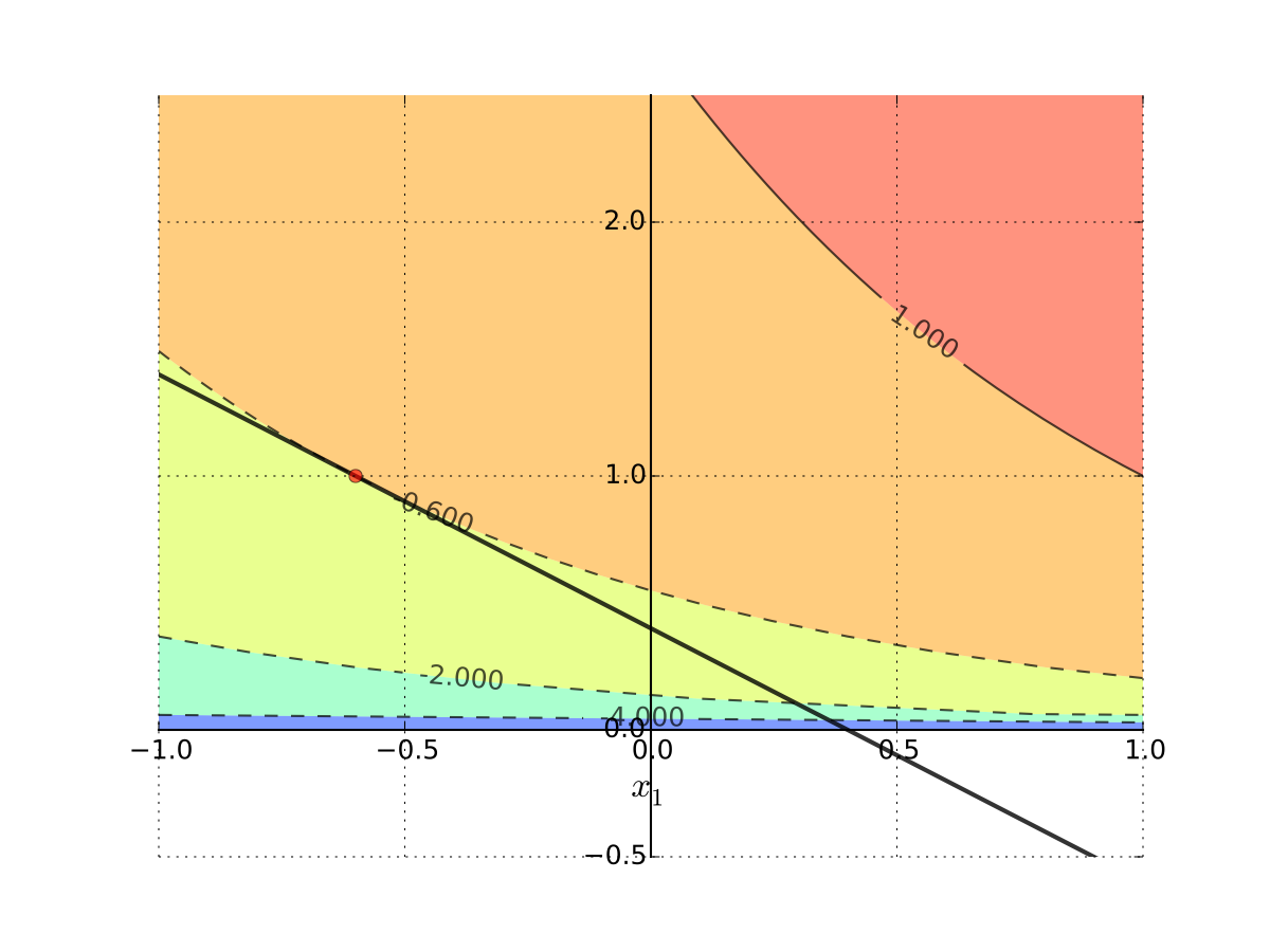
Fig. 77 Tangent point is infeasible

Interpretation: No interior solution

Put differently

• Every interior point on the budget line is dominated by the infeasible solution

• Hence solution must be on the boundary

Since \(x_2 = 0\) implies \(x_1 + \log(x_2) = - \infty\), solution is

• \(x_1^\star = 0\)

• \(x_2^\star = m/p_2 = 0.4\)

Fig. 78 Corner solution

Let’s look at the systematic solution approach where the corner solutions will emerge naturally when they are optimal.

Karush-Kuhn-Tucker conditions

Fact (Karush-Kuhn-Tucker conditions for maximization)

Let \(f \colon \mathbb{R}^N \to \mathbb{R}\) and \(g \colon \mathbb{R}^N \to \mathbb{R}^K\) be continuously differentiable functions.

Let \(D = \{ x \colon g_i(x) \le 0, i=1,\dots,K \} \subset \mathbb{R}^N\)

Suppose that

• \(x^\star \in D\) is a local maximum of \(f\) on \(D\), and

• the gradients of the constraint functions \(g_i\) corresponding to the binding constraints are linearly independent at \(x^\star\) (equivalently, the rank of the matrix composed of the gradients of the binding constraints is equal to the number of binding constraints).

Then there exists a vector \(\lambda^\star \in \mathbb{R}^K\) such that

\[ Df(x^\star) - \lambda^\star \cdot Dg(x^\star) = Df(x^\star) - \sum_{i=1}^K \lambda_i^\star Dg_i(x^\star) = 0 \]

and

\[\begin{split} \begin{cases} \lambda_i^\star \ge 0, \\ \lambda_i^\star g_i(x^\star) = 0 \; i=1,\dots,K \end{cases} \end{split}\]

Proof

See Sundaram 6.5

• Compare to the Lagrange theorem for equality constraints: what is the difference?

Karush-Kuhn-Tucker conditions (miminization)

In the settings of KKT conditions (maximization), suppose that \(x^\star \in D\) is a local minimum of \(f\) on \(D\), and as before the matrix composed of the gradients of the binding constraints has full rank.

Then there exists a vector \(\lambda^\star \in \mathbb{R}^K\) such that (note opposite sign)

\[ Df(x^\star) + \lambda^\star \cdot Dg(x^\star) = Df(x^\star) + \sum_{i=1}^K \lambda_i^\star Dg_i(x^\star) = 0 \]

and

\[\begin{split} \begin{cases} \lambda_i^\star \ge 0, \\ \lambda_i^\star g_i(x^\star) = 0 \; i=1,\dots,K \end{cases} \end{split}\]

• Very similar to the Lagrange theorem, but now we have inequalities!

• The last set of conditions is called the complementary slackness conditions, and they play the following role:

  • if for a given \(i\) \(g_i(x^\star) = 0\), that is the \(i\)-th constraint is binding , then the corresponding \(\lambda_i^\star > 0\) acts as a Lagrange multiplier for an equality constraint

  • if on the other hand for a given \(i\) \(g_i(x^\star) < 0\), the corresponding \(\lambda_i^\star\) must be zero, removing the term with \(Dg_i(x^\star)\) from the first condition

• This way the KKT conditions combine the unconstrained and equality constrained conditions in one

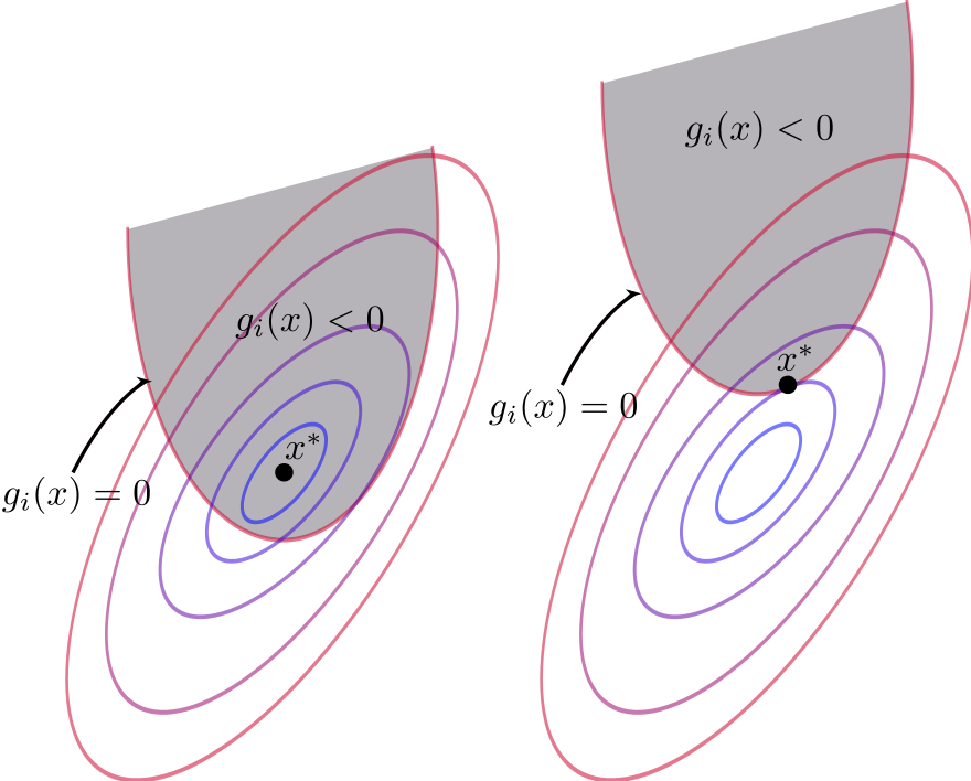
Fig. 79 Binding and non-binding constraint at \(x^\star\)

Karush - Kuhn-Tucker method: recipe

Essentially the same as for the Lagrange method

Combination of the unconstrained and equality constrained optimization algorithms

1. Write down the Lagrangian function \(\mathcal{L}(x,\lambda)\)

2. Write down KKT conditions as a system of first order conditions on \(\mathcal{L}(x,\lambda)\) together with the non-negativity of \(\lambda\) and complementary slackness conditions

3. Systematically consider all \(2^K\) combinations of binding and non-binding constraints, solving the simplified system of KKT conditions in each case to find the candidate stationary points. Don’t forget to check the found solutions against the conditions defining each case

4. To check the second order conditions, apply the theory of unconstrained or constrained optimization as appropriate to the relevant set of the binding constraints

5. To find the global optima, compare the function values at all identified local optima

Possible issues with KKT method are similar to the Lagrange method:

• constraint qualification assumption

• existence of constrained optima

• local vs global optimality

Example

Returning to the utility maximization problem with budget constraint and non-negative consumption

\[\begin{split} u(x_1, x_2) = \alpha x_1 + \beta \log(x_2) \to \max_{x_1, x_2} \\ \text{ subject to} \\ p_1 x_1 + p_2 x_2 \leq m \\ x_1 \geq 0, \; x_2 \geq 0 \end{split}\]

Form the Lagrangian with 3 inequality constraints (have to flip the sign for non-negativity to stay within the general formulation)

\[\begin{split} \mathcal{L}(x_1,x_2,\lambda_1,\lambda_2,\lambda_3) = \\ = \alpha x_1 + \beta\log(x_2) - \lambda_1 (-x_1) - \lambda_2 (-x_2) - \lambda_3 (p_1 x_1 + p_2 x_2 -m) = \\ = \alpha x_1 + \beta\log(x_2) + \lambda_1 x_1+ \lambda_2 x_2 - \lambda_3 (p_1 x_1 + p_2 x_2 -m) \end{split}\]

The necessary KKT conditions are given by the following system of equations

\[\begin{split} \begin{cases} \frac{\partial \mathcal{L}}{\partial x_1} = 0 \implies \alpha + \lambda_1 - \lambda_3 p_1 = 0 \\ \frac{\partial \mathcal{L}}{\partial x_2} = 0 \implies \frac{\beta}{x_2} + \lambda_2 - \lambda_3 p_2 = 0 \\ x_1 \ge 0 \\ x_2 \ge 0 \\ x_1 p_1 + x_2 p_2 \le m \\ \lambda_1 \ge 0 \text { and } \lambda_1 x_1 = 0 \\ \lambda_2 \ge 0 \text { and } \lambda_2 x_2 = 0 \\ \lambda_3 \ge 0 \text { and } \lambda_3 (x_1 p_1 + x_2 p_2 -m) = 0 \\ \end{cases} \end{split}\]

The KKT conditions can be solved systematically by considering all combinations of the multipliers:

1. \(\lambda_1=\lambda_2=\lambda_3=0\)
   The first equation becomes \(\alpha = 0\) which is inconsistent with the initially set \(\alpha>0\)

2. \(\lambda_1=\lambda_2=0, \; \lambda_3>0 \implies x_1 p_1 + x_2 p_2 -m = 0\)
   This is the exact case we looked at with the Lagrange method ignoring the non-negativity conditions on consumption. The solution is \(x_1^\star = \frac{m}{p_1} - \frac{\beta}{\alpha}\) and \(x_2^\star = \frac{\beta p_1}{\alpha p_2}\) if it also holds that \(x_1^\star \ge 0\) and \(x_2^\star \ge 0\), i.e. \(p_1/m \le \alpha/\beta\)

3. \(\lambda_1=\lambda_3=0, \; \lambda_2>0 \implies x_2 = 0\)
   The case of \(x_2=0\) is outside of the domain of the utility function and could in fact be excluded from the start.

4. \(\lambda_1=0, \;\lambda_2>0, \; \lambda_3>0 \implies x_2 = 0\) and \(p_1 + x_2 p_2 -m = 0\)
   Inconsistent similarly to the previous case

5. \(\lambda_1>0, \;\lambda_2 = \lambda_3 = 0 \implies x_1 = 0\)
   The second equation becomes \(\beta / x_2 = 0\) which is inconsistent with the \(\beta>0\) and \(x_2 \ne 0\)

6. \(\lambda_1>0, \;\lambda_2 = 0, \; \lambda_3 > 0 \implies x_1 = 0\) and \(p_1 + x_2 p_2 -m = 0\)
   We have the following system in this case

\[\begin{split} \begin{cases} \alpha + \lambda_1 - \lambda_3 p_1 = 0 \\ \frac{\beta}{x_2} - \lambda_3 p_2 = 0 \\ x_2 p_2 -m = 0 \end{cases} \end{split}\]

From the last equation \(x_2 = m/p_2\), combining the two last equations \(\lambda_3 = \beta/m\), and from the first equation \(\lambda_1 = \beta p_1/m - \alpha\). The solution holds conditional on \(\lambda_1>0\), i.e. \(p_1/m > \alpha/\beta\).

7. \(\lambda_1>0, \;\lambda_2 > 0, \; \lambda_3 = 0 \implies x_1 = 0\) and \(x_2 = 0\)
   Inconsistent similar to case 3

8. \(\lambda_1>0, \;\lambda_2 > 0, \; \lambda_3 > 0 \implies x_1 = x_2 = p_1 + x_2 p_2 -m = 0\)
   Inconsistent similarly to the previous case

To summarize, the solution to the KKT conditions is given by the following cases (it’s easy to see that the two solutions coincide for the equality in the parameter condition):

\[\begin{split} \begin{cases} x_1^\star = \frac{m}{p_1} - \frac{\beta}{\alpha}, \; x_2^\star = \frac{\beta p_1}{\alpha p_2}, & \text{ if } p_1/m \le \alpha/\beta, \\ x_1^\star = 0, \; x_2^\star = \frac{m}{p_2}, & \text{ if } p_1/m > \alpha/\beta \\ \end{cases} \end{split}\]

Thus, the corner solution is included in the solution set of the KKT conditions.

Second order conditions

Note that KKT conditions are essentially necessary first order conditions, similarly to the Lagrange theorem.

What about the necessary or sufficient second order conditions?

Either the unconstrained second order conditions or the equality constrained second order conditions have to be applied depending on the considered combination of the binding and non-binding constraints.

See the relevant sections in the previous lectures:

• unconstrained necessary and sufficient SOC

• constrained necessary and sufficient SOC

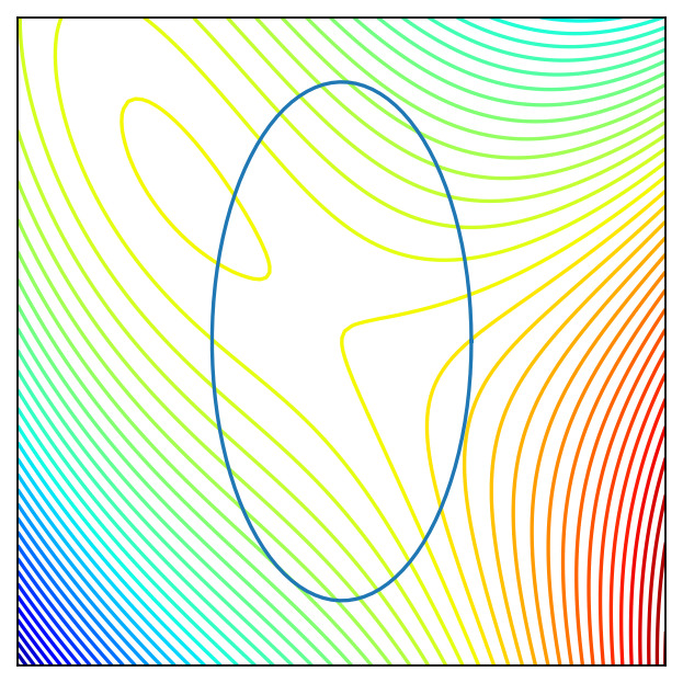
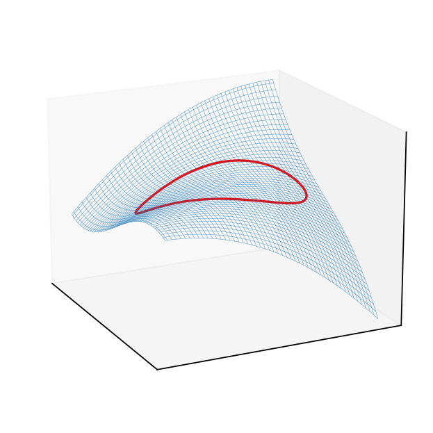
Example

\[\begin{split} f(x,y) = x^2+y^2 \to \max_{x,y} \\ \text {subject to} \\ \begin{cases} (y+1)^3 \geqslant x^2,\\ x^2 + y \leqslant 1\\ \end{cases} \end{split}\]

---

Solution:

Show code cell content Hide code cell content

import numpy as np
import matplotlib.pyplot as plt
from mpl_toolkits.mplot3d import Axes3D
from matplotlib import cm
from myst_nb import glue

f = lambda x: x[0]**3/3 - 3*x[1]**2 + 5*x[0] - 6*x[0]*x[1]

x = y = np.linspace(-10.0, 10.0, 100)
X, Y = np.meshgrid(x, y)
zs = np.array([f((x,y)) for x,y in zip(np.ravel(X), np.ravel(Y))])
Z = zs.reshape(X.shape)

a,b=4,8
# (x/a)^2 + (y/b)^2 = 1
theta = np.linspace(0, 2 * np.pi, 100)
X1 = a*np.cos(theta)
Y1 = b*np.sin(theta)
zs = np.array([f((x,y)) for x,y in zip(np.ravel(X1), np.ravel(Y1))])
Z1 = zs.reshape(X1.shape)

fig = plt.figure(dpi=160)
ax2 = fig.add_subplot(111)
ax2.set_aspect('equal', 'box')
ax2.contour(X, Y, Z, 50,
            cmap=cm.jet)
ax2.plot(X1, Y1)
plt.setp(ax2, xticks=[],yticks=[])
glue("example_problem_1", fig, display=False)

fig = plt.figure(dpi=160)
ax3 = fig.add_subplot(111, projection='3d')
ax3.plot_wireframe(X, Y, Z, 
            rstride=2, 
            cstride=2,
            alpha=0.7,
            linewidth=0.25)
f0 = f(np.zeros((2)))+0.1
ax3.plot(X1, Y1, Z1, c='red')
plt.setp(ax3,xticks=[],yticks=[],zticks=[])
ax3.view_init(elev=18, azim=154)
glue("example_problem_2", fig, display=False)

Example

\[\begin{split} f(x,y) = \frac{x^3}{3}-3y^2+5x-6xy \to \max_{x,y} \\ \text {subject to} \\ (x/4)^2 + (y/8)^2 \le 1,\\ x,y \in \mathbb{R} \end{split}\]

How many ``cases’’ do we expect to consider?