📚 Revision: matrix arithmetic

⏱ | words

References and additional materials

[Simon and Blume, 1994]

Chapters 8, 9

Matrix

Definition

A matrix is an array of numbers or variables which are organised into rows and columns

An \((n \times m)\) matrix takes the following form:

\[\begin{split} A=\left(\begin{array}{ccccc} a_{11} & a_{12} & a_{13} & \cdots & a_{1 m} \\ a_{21} & a_{22} & a_{23} & \cdots & a_{2 m} \\ a_{31} & a_{32} & a_{33} & \cdots & a_{3 m} \\ \vdots & \vdots & \vdots & \ddots & \vdots \\ a_{n 1} & a_{n 2} & a_{n 3} & \cdots & a_{n m} \end{array}\right) \end{split}\]

• \(n\) and \(m\) are dimensions of the matrix A

An \((n \times m)\) matrix has \(n\) rows and \(m\) columns

Note that, while it is possible that \(n=m\), it is also possible that \(n \neq m\)

Definition

Matrix with has the same number of column as rows, \(n=m\), is called a square matrix.

Scalars and vectors

Definition

A scalar is a real number \((a \in \mathbb{R})\)

Definition

A column vector is an \((n \times 1)\) matrix of the form

\[\begin{split} A=\left(\begin{array}{c} a_{11} \\ a_{21} \\ a_{31} \\ \vdots \\ a_{n 1} \end{array}\right) \end{split}\]

A row vector is a \((1 \times m)\) matrix of the form

\[ A=\left(\begin{array}{lllll} a_{11} & a_{12} & a_{13} & \cdots & a_{1 m} \end{array}\right) . \]

• Vectors can be thought of as matrixes with one dimension equal to \(1\)

• Scalars can be thought of as \(1 \times 1\) matrixes

Matrix arithmetic

• Scalar multiplication of a matrix

• Matrix addition

• Matrix subtraction

• Matrix multiplication: The inner, or dot, product

• The transpose of a matrix and matrix symmetry

• The additive inverse of a matrix and the null matrix

• The multiplicative inverse of a matrix and the identity matrix

Note

Many binary operations with matrices are not commutative! (order of operands is important)

Let \(A\) is an \((n \times m)\) matrix takes the following form:

\[\begin{split} A=\left(\begin{array}{ccccc} a_{11} & a_{12} & a_{13} & \cdots & a_{1 m} \\ a_{21} & a_{22} & a_{23} & \cdots & a_{2 m} \\ a_{31} & a_{32} & a_{33} & \cdots & a_{3 m} \\ \vdots & \vdots & \vdots & \ddots & \vdots \\ a_{n 1} & a_{n 2} & a_{n 3} & \cdots & a_{n m} \end{array}\right) \end{split}\]

We will assume that \(a_{i j} \in \mathbb{R}\) for all

\[ (i, j) \in\{1,2, \cdots, n\} \times\{1,2, \cdots, m\} . \]

Scalar multiplication

Suppose that \(c \in \mathbb{R}\). The scalar pre-product and post-product of this constant with this matrix is given by

\[\begin{split} c A & = A c = \left(\begin{array}{ccccc} c a_{11} & c a_{12} & c a_{13} & \cdots & c a_{1 m} \\ c a_{21} & c a_{22} & c a_{23} & \cdots & c a_{2 m} \\ c a_{31} & c a_{32} & c a_{33} & \cdots & c a_{3 m} \\ \vdots & \vdots & \vdots & \ddots & \vdots \\ c a_{n 1} & c a_{n 2} & c a_{n 3} & \cdots & c a_{n m} \end{array}\right) \end{split}\]

Note that \(c A=A c\). As such, we can just talk about the scalar product of a constant with a matrix, without specifying the order in which the multiplication takes place.

Examples

\[\begin{split} 2\left(\begin{array}{ll} 1 & 1 \\ 1 & 2 \end{array}\right)=\left(\begin{array}{ll} 2\cdot1 & 2\cdot1 \\ 2\cdot1 & 2\cdot2 \end{array}\right)=\left(\begin{array}{ll} 2 & 2 \\ 2 & 4 \end{array}\right) \end{split}\]

\[\begin{split} 2\left(\begin{array}{cc} -1 & -2 \\ 3 & 1 \end{array}\right)=\left(\begin{array}{cc} 2\cdot(-1) & 2\cdot(-2) \\ 2\cdot3 & 2\cdot1 \end{array}\right)=\left(\begin{array}{cc} -2 & -4 \\ 6 & 2 \end{array}\right) \end{split}\]

\[\begin{split} \left(\begin{array}{ccc} 1 & 2 & 0 \\ 4 & -3 & 1 \end{array}\right) \cdot 2 =\left(\begin{array}{ccc} 3 & 6 & 0 \\ 12 & -9 & 3 \end{array}\right) \end{split}\]

\[\begin{split} -\frac{1}{2}\left(\begin{array}{lll} 0 & 1 & 2 \\ 1 & 0 & 2 \end{array}\right)= & =\left(\begin{array}{ccc} 0 & -\tfrac{1}{2} & -1 \\ -\tfrac{1}{2} & 0 & -1 \end{array}\right) \end{split}\]

Matrix addition

The sum of two matrices is only defined if the two matrices have exactly the same dimensions.

Definition

Two matrixes are called conformable for a given operation if their dimensions are such that the operation is well defined.

Suppose that \(B\) is an \((n \times m)\) matrix that takes the following form:

\[\begin{split} B=\left(\begin{array}{ccccc} b_{11} & b_{12} & b_{13} & \cdots & b_{1 m} \\ b_{21} & b_{22} & b_{23} & \cdots & b_{2 m} \\ b_{31} & b_{32} & b_{33} & \cdots & b_{3 m} \\ \vdots & \vdots & \vdots & \ddots & \vdots \\ b_{n 1} & b_{n 2} & b_{n 3} & \cdots & b_{n m} \end{array}\right) \end{split}\]

The matrix sum \((A+B)\) is an \((n \times m)\) matrix that takes the following form:

\[\begin{split} A+B = B+A =\left(\begin{array}{cccc} a_{11}+b_{11} & a_{12}+b_{12} & \cdots & a_{1 m}+b_{1 m} \\ a_{21}+b_{21} & a_{22}+b_{22} & \cdots & a_{2 m}+b_{2 m} \\ \vdots & \vdots & \ddots & \vdots \\ a_{n 1}+b_{n 1} & a_{n 2}+b_{n 2} & \cdots & a_{n m}+b_{n m} \end{array}\right) \end{split}\]

Note matrix summation is also commutative, \(A+B=B+A\).

Exercise: Convince yourself in this fact.

Examples

\[\begin{split} \left(\begin{array}{ll} 1 & 1 \\ 1 & 2 \end{array}\right)+\left(\begin{array}{ll} 1 & 0 \\ 1 & 2 \end{array}\right)=\left(\begin{array}{ll} 1+1 & 1+0 \\ 1+1 & 2+2 \end{array}\right)=\left(\begin{array}{ll} 2 & 1 \\ 2 & 4 \end{array}\right) \end{split}\]

\[\begin{split} \left(\begin{array}{ll} 1 & 1 \\ 1 & 2 \end{array}\right)+\left(\begin{array}{ll} -1 & 3 \\ -2 & 1 \end{array}\right)=\left(\begin{array}{ll} 1+(-1) & 1+3 \\ 1+(-2) & 2+1 \end{array}\right) =\left(\begin{array}{cc} 0 & 4 \\ -1 & 3 \end{array}\right) \end{split}\]

\[\begin{split} \begin{gathered} \left(\begin{array}{ccc} 1 & 2 & 0 \\ 4 & -3 & -1 \end{array}\right)+\left(\begin{array}{lll} 0 & 1 & 2 \\ 1 & 0 & 2 \end{array}\right) =\left(\begin{array}{ccc} 1 & 3 & 2 \\ 5 & -3 & 1 \end{array}\right) \end{gathered} \end{split}\]

Matrix subtraction

Matrix subtraction involves a combination of (i) scalar multiplication of a matrix, and (ii) matrix addition.

As with matrix addition, the difference of two matrices is only defined if the two matrices have exactly the same dimensions.

Suppose that \(A\) and \(B\) are both \((n \times m)\) matrices. The difference between \(A\) and \(B\) is defined to be

\[ A-B=A+(-1) B \]

In general, \(A-B \neq B-A\)

Example

Under what circumstances will \(A-B=B-A\) ?

Solution

\[\begin{split}A-B = B-A \\ A = B - A + B \\ A + A = B + B \\ 2A = 2B \\ A = B\end{split}\]

We can work with matrices as variables in the equation!

Matrix multiplication

• The standard matrix product is the dot, or inner, product of two matrices.

• The dot product of two matrices is only defined for cases in which the number of columns of the first listed matrix is identical to the number of rows of the second listed matrix.

• If the dot product is defined, the solution matrix will have the same number of rows as the first listed matrix and the same number of columns as the second listed matrix.

Let \(B\) be an \((m \times p)\) matrix that takes the following form:

\[\begin{split} B=\left(\begin{array}{ccccc} b_{11} & b_{12} & b_{13} & \cdots & b_{1 p} \\ b_{21} & b_{22} & b_{23} & \cdots & b_{2 p} \\ b_{31} & b_{32} & b_{33} & \cdots & b_{3 p} \\ \vdots & \vdots & \vdots & \ddots & \vdots \\ b_{m 1} & b_{m 2} & b_{m 3} & \cdots & b_{m p} \end{array}\right) \end{split}\]

The matrix product \(A B\) is defined and will be an \((n \times p)\) matrix. The solution matrix is given by

\[\begin{split} \begin{array}{rl} AB &=\left(\begin{array}{cccc} a_{11} & a_{12} & \cdots & a_{1 m} \\ a_{21} & a_{22} & \cdots & a_{2 m} \\ \vdots & \vdots & \ddots & \vdots \\ a_{n 1} & a_{n 2} & \cdots & a_{n m} \end{array}\right) \cdot\left(\begin{array}{cccc} b_{11} & b_{12} & \cdots & b_{1 p} \\ b_{21} & b_{22} & \cdots & b_{2 p} \\ \vdots & \vdots & \ddots & \vdots \\ b_{m 1} & b_{m 2} & \cdots & b_{m p} \end{array}\right) \\[20pt] &=\left(\begin{array}{ccccc} \sum_{k=1}^{m} a_{1 k} b_{k 1} & \sum_{k=1}^{m} a_{1 k} b_{k 2} & \cdots & \sum_{k=1}^{m} a_{1 k} b_{k p} \\ \sum_{k=1}^{m} a_{2 k} b_{k 1} & \sum_{k=1}^{m} a_{2 k} b_{k 2} & \cdots & \sum_{k=1}^{m} a_{2 k} b_{k p} \\ \vdots & \vdots & \ddots & \vdots \\ \sum_{k=1}^{m} a_{n k} b_{k 1} & \sum_{k=1}^{m} a_{n k} b_{k 2} & \cdots & \sum_{k=1}^{m} a_{n k} b_{k p} \end{array}\right) \end{array} \end{split}\]

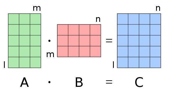
Fig. 22 Matrix multiplication: conformable matrices

Definition

A dot product of two vectors \(x = (x_1,\dots,x_N) \in \mathbb{R}^N\) and \(y = (y_1,\dots,y_N) \in \mathbb{R}^N\) is given by

\[x \cdot y = \sum_{i=1}^N x_i y_i\]

Fig. 23 Matrix multiplication: combination of dot products of vectors

Fact

Matrix multiplication is not commutative in general

\[ A B \neq B A \]

Example

\[\begin{split} \begin{array}{l} \left(\begin{array}{cc} 1 & 2 \\ -2 & 4 \end{array}\right) \cdot\left(\begin{array}{lll} 0 & 2 & 2 \\ 1 & 0 & 5 \end{array}\right) \\ =\left(\begin{array}{ccc} (1)(0)+(2)(1) & (1)(2)+(2)(0) & (1)(2)+(2)(5) \\ (-2)(0)+(4)(1) & (-2)(2)+(4)(0) & (-2)(2)+(4)(5) \end{array}\right) \\ =\left(\begin{array}{ccc} 0+2 & 2+0 & 2+10 \\ 0+4 & -4+0 & -4+20 \end{array}\right) \\ =\left(\begin{array}{ccc} 2 & 2 & 12 \\ 4 & -4 & 16 \end{array}\right) \end{array} \end{split}\]

\[\begin{split} \begin{aligned} A C &=\left(\begin{array}{cc} 1 & 2 \\ -2 & 4 \end{array}\right) \cdot\left(\begin{array}{cc} 3 & -2 \\ 5 & 0 \end{array}\right) \\ &=\left(\begin{array}{cc} (1)(3)+(2)(5) & (1)(-2)+(2)(0) \\ (-2)(3)+(4)(5) & (-2)(-2)+(4)(0) \end{array}\right) \\ &=\left(\begin{array}{cc} 3+10 & -2+0 \\ -6+20 & 4+0 \end{array}\right) \\ &=\left(\begin{array}{cc} 13 & -2 \\ 14 & 4 \end{array}\right) \end{aligned} \end{split}\]

\[\begin{split} \begin{aligned} C A &=\left(\begin{array}{cc} 3 & -2 \\ 5 & 0 \end{array}\right) \cdot\left(\begin{array}{cc} 1 & 2 \\ -2 & 4 \end{array}\right) \\ &=\left(\begin{array}{cc} (3)(1)+(-2)(-2) & (3)(2)+(-2)(4) \\ (5)(1)+(0)(-2) & (5)(2)+(0)(4) \end{array}\right) \\ &=\left(\begin{array}{cc} 3+4 & 6+(-8) \\ 5+0 & 10+0 \end{array}\right) \\ &=\left(\begin{array}{cc} 7 & -2 \\ 5 & 10 \end{array}\right) \end{aligned} \end{split}\]

Note that \(A C \neq C A\).

Note

Do not confuse various names for the two types of matrix/vector multiplication:

Dot/scalar/inner product denoted with a dot \(\cdot\) is the sum of products of the vector coordinates, outputs a scalar

Vector/cross product denoted with a cross \(\times\) is a vector that is orthogonal to the two input vectors with a length equal to the area of the parallelogram spanned by the two input vectors (not covered in this course)

Matrix transposition

Suppose that \(A\) is an \((n \times m)\) matrix. The transpose of the matrix \(A\), which is denoted by \(A^{T}\), is the \((m \times n)\) matrix that is formed by taking the rows of \(A\) and turning them into columns, without changing their order. In other words, the \(i\) th column of \(A^{T}\) is the ith row of \(A\). This also means that the jth row of \(A^{T}\) is the \(j\) th column of \(A\).

The transpose of the matrix \(A\) is the \((m \times n)\) matrix that takes the following form:

\[\begin{split} A=\left(\begin{array}{ccccc} a_{11} & a_{12} & a_{13} & \cdots & a_{1 m} \\ a_{21} & a_{22} & a_{23} & \cdots & a_{2 m} \\ a_{31} & a_{32} & a_{33} & \cdots & a_{3 m} \\ \vdots & \vdots & \vdots & \ddots & \vdots \\ a_{n 1} & a_{n 2} & a_{n 3} & \cdots & a_{n m} \end{array}\right) \quad A^{T}=\left(\begin{array}{ccccc} a_{11} & a_{21} & a_{31} & \cdots & a_{n 1} \\ a_{12} & a_{22} & a_{32} & \cdots & a_{n 2} \\ a_{13} & a_{23} & a_{33} & \cdots & a_{n 3} \\ \vdots & \vdots & \vdots & \ddots & \vdots \\ a_{1 m} & a_{2 m} & a_{3 m} & \cdots & a_{n m} \end{array}\right) \end{split}\]

Examples

• If \( x=\left(\begin{array}{l} 1 \\ 3 \\ 5 \end{array}\right) \) then \(X^{T}=(1,3,5)\).
  
  
  

• If \( Y=\left(\begin{array}{ll} 2 & 3 \\ 5 & 9 \\ 7 & 6 \end{array}\right) \) then \( Y^{T}=\left(\begin{array}{lll} 2 & 5 & 7 \\ 3 & 9 & 6 \end{array}\right) \).
  
  
  

• If \( Z=\left(\begin{array}{ccc} 1 & 3 & 7 \\ 4 & 5 & 11 \\ 6 & 8 & 10 \end{array}\right) \) then \( Z^{T}=\left(\begin{array}{ccc} 1 & 4 & 6 \\ 3 & 5 & 8 \\ 7 & 11 & 10 \end{array}\right) \).

In general, \(A^{T} \neq A\).

Definition

If matrix \(A\) is such that \(A^{T}=A\), we say that \(A\) is a symmetric matrix.

Example

\( A=\left(\begin{array}{ll} 0 & 0 \\ 0 & 0 \end{array}\right)=A^{T} \)

\( B=\left(\begin{array}{ll} 1 & 0 \\ 0 & 1 \end{array}\right)=B^{T} \)

\( C=\left(\begin{array}{ll} 0 & 1 \\ 1 & 0 \end{array}\right)=C^{T} \)

\( D=\left(\begin{array}{ll} 1 & 0 \\ 0 & 0 \end{array}\right)=D^{T} \)

Fact

If \(A\) and \(B\) are conformable for matrix multiplication, then

\[(AB)^{T} = B^T A^T\]

Null matrices

Definition

A null matrix (or vector) is a matrix that consists solely of zeroes.

Example

For example, the \((3 \times 3)\) null matrix is

\[\begin{split} \mathbb{0}= \left(\begin{array}{ccc} 0 & 0 & 0 \\ 0 & 0 & 0 \\ 0 & 0 & 0 \end{array}\right) \end{split}\]

Fact

For an \((n \times m)\) null matrix and an \((n \times m)\) matrix \(A\), it holds \(A+0=0+A=A\).

Definition

Suppose that \(A\) is an \((n \times m)\) matrix and \(\mathbb{0}\) is the \((n \times m)\) null matrix. The \((n \times m)\) matrix \(B\) is called the additive inverse of \(A\) if and only if \(A+B=B+A=0\).

The additive inverse of \(A\) is

\[\begin{split} B=-A=\left(\begin{array}{cccc} -a_{11} & -a_{12} & \cdots & -a_{1 m} \\ -a_{21} & -a_{22} & \cdots & -a_{2 m} \\ \vdots & \vdots & \ddots & \vdots \\ -a_{n 1} & -a_{n 2} & \cdots & -a_{n m} \end{array}\right) \end{split}\]

Fact

\[ \left( A^T \right)^T = A \]

Identity matrices

Definition

An identity matrix is a square matrix that has ones on the main (north-west to south-east) diagonal and zeros everywhere else.

Example

For example, the \((2 \times 2)\) identity matrix is

\[\begin{split} I=\left(\begin{array}{ll} 1 & 0 \\ 0 & 1 \end{array}\right) \end{split}\]

Fact

For an \((n \times n)\) identity matrix \(I\) it holds:

• If \(A\) is an \((n \times n)\) matrix, then \(A I=I A=A\).

• If \(A\) is an \((m \times n)\) matrix, then \(A I=A\).

• If \(A\) is an \((n \times m)\) matrix, then \(I A=A\).

Definition

Let \(A\) be an \((n \times n)\) matrix and \(I\) be the \((n \times n)\) identity matrix. The \((n \times n)\) matrix \(B\) is the multiplicative inverse (usually just referred to as the inverse) of \(A\) if and only if \(A B=B A=I\).

• Only square matrices have any chance of having a multiplicative inverse

• Some, but not all, square matrices will have a multiplicative inverse

Definition

• A square matrix that has an inverse is said to be non-singular.

• A square matrix that does not have an inverse is said to be singular.

• We will talk about methods for determining whether or not a matrix is non-singular later in this course

Fact

The transpose of the inverse is equal to the inverse of the transpose

If \(A\) is a non-singular square matrix whose multiplicative inverse is \(A^{-1}\), then we have

\[\left(A^{-1}\right)^{T}=\left(A^{T}\right)^{-1}\]

Example

Note that

\[\begin{split} \begin{aligned} A B &=\left(\begin{array}{ll} 1 & 2 \\ 3 & 7 \end{array}\right) \cdot\left(\begin{array}{cc} 7 & -2 \\ -3 & 1 \end{array}\right) \\[10pt] &=\left(\begin{array}{cc} (1)(7)+(2)(-3) & (1)(-2)+(2)(1) \\ (3)(7)+(7)(-3) & (3)(-2)+(7)(1) \end{array}\right) \\[10pt] &=\left(\begin{array}{cc} 7+(-6) & -2+2 \\ 21+(-21) & -6+7 \end{array}\right) \\[10pt] &=\left(\begin{array}{ll} 1 & 0 \\ 0 & 1 \end{array}\right) \\[10pt] &= I \end{aligned} \end{split}\]

Note that

\[\begin{split} \begin{aligned} B A &=\left(\begin{array}{cc} 7 & -2 \\ -3 & 1 \end{array}\right) \cdot\left(\begin{array}{cc} 1 & 2 \\ 3 & 7 \end{array}\right) \\[10pt] &=\left(\begin{array}{cc} (7)(1)+(-2)(3) & (7)(2)+(-2)(7) \\ (-3)(1)+(1)(3) & (-3)(2)+(1)(7) \end{array}\right) \\[10pt] &=\left(\begin{array}{cc} 7+(-6) & 14+(-14) \\ -3+3 & -6+7 \end{array}\right) \\[10pt] &=\left(\begin{array}{cc} 1 & 0 \\ 0 & 1 \end{array}\right) \\[10pt] &= I \end{aligned} \end{split}\]

Since \(A B=B A=I\), we can conclude that \(A^{-1}=B\).

[Haeussler Jr and Paul, 1987] (p. 278, Example 1)

Determinants

Determinant is a fundamental characteristic of any matrix \(A\) and a linear operator given by a matrix \(A\)

Note

Determinants are only defined for square matrices, so in this section we only consider square matrices.

• we use some sort of recursive definition

Definition

For a square \(2 \times 2\) matrix the determinant is given by

\[\begin{split} % \det \left( \begin{array}{cc} a & b \\ c & d \\ \end{array} \right) = ad - bc % \end{split}\]

Notation for the determinant is either \(\det(A)\) or sometimes \(|A|\)

Example

\[\begin{split} % \det \left( \begin{array}{cc} 2 & 0 \\ 7 & -1 \\ \end{array} \right) = (2 \times -1) - (7 \times 0) = -2 % \end{split}\]

We build the definition of the determinants of larger matrices from \(2 \times 2\) case. Think of the next definitions as a ‘induction step’

Definition

Consider an \(n \times n\) matrix \(A\). Denote \(A_{ij}\) a \((n-1) \times (n-1)\) submatrix of \(A\), obtained by deleting the \(i\)-th row and \(j\)-th column of \(A\). Then

• the \((i,j)\)-th minor of \(A\) denoted \(M_{ij}\) is

\[ M_{ij} = \det(A_{ij}) \]

• the \((i,j)\)-th cofactor of \(A\) denoted \(C_{ij}\)

\[ C_{ij} = (-1)^{i+j} M_{ij} = (-1)^{i+j} \det(A_{ij}) \]

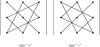
• cofactors are signed minors

• signs alternate in checkerboard pattern

\[\begin{split} \left[\; \begin{array}{cccccc} + & - & + & - & + & \dots \\ - & + & - & + & - & \dots \\ + & - & + & - & + & \dots \\ - & + & - & + & - & \dots \\ + & - & + & - & + & \dots \\ \vdots & \vdots & \vdots & \vdots & \vdots & \ddots \end{array} \;\right] \end{split}\]

• for even \(i+j\) minors and cofactors are equal

Definition

The determinant of an \(n \times n\) matrix \(A\) with elements \(\{a_{ij}\}\) is given by

\[ \det(A) = \sum_{i=1}^n a_{ij} C_{ij} = \sum_{j=1}^n a_{ij} C_{ij} \]

for any choice of \(i\) or \(j\).

• given that the cofactors are lower dimension determinants, we can use the same formula to compute determinants of matrices of all sizes

Example

Expanding along the first column:

\[\begin{split} \begin{array}{l} \left| \begin{array}{ccc} a_{11},& a_{12},& a_{13} \\ a_{21},& a_{22},& a_{23} \\ a_{31},& a_{32},& a_{33} \end{array} \right| = a_{11} \left| \begin{array}{ccc} a_{22},& a_{23} \\ a_{32},& a_{33} \end{array} \right| + (-1)^3 a_{21} \left| \begin{array}{ccc} a_{12},& a_{13} \\ a_{32},& a_{33} \end{array} \right| + a_{31} \left| \begin{array}{ccc} a_{12},& a_{13} \\ a_{22},& a_{23} \end{array} \right| = \\ = a_{11} (a_{22}a_{33} - a_{23}a_{32}) - a_{21} (a_{12}a_{33}-a_{13}a_{32}) + a_{31} (a_{12}a_{23}-a_{13}a_{22}) = \\ = a_{11} a_{22}a_{33} + a_{21}a_{13}a_{32} + a_{31}a_{12}a_{23} - a_{11}a_{23}a_{32} - a_{21}a_{12}a_{33} - a_{31}a_{13}a_{22} \end{array} \end{split}\]

Expanding along the top row:

\[\begin{split} \begin{array}{l} \left| \begin{array}{ccc} a_{11},& a_{12},& a_{13} \\ a_{21},& a_{22},& a_{23} \\ a_{31},& a_{32},& a_{33} \end{array} \right| = a_{11} \left| \begin{array}{ccc} a_{22},& a_{23} \\ a_{32},& a_{33} \end{array} \right| + (-1)^3 a_{12} \left| \begin{array}{ccc} a_{21},& a_{23} \\ a_{31},& a_{33} \end{array} \right| + a_{13} \left| \begin{array}{ccc} a_{21},& a_{22} \\ a_{31},& a_{32} \end{array} \right| = \\ = a_{11} (a_{22}a_{33} - a_{23}a_{32}) - a_{12} (a_{21}a_{33}-a_{23}a_{31}) + a_{13} (a_{21}a_{32}-a_{22}a_{31}) = \\ = a_{11} a_{22}a_{33} + a_{12}a_{23}a_{31} + a_{13}a_{21}a_{32} - a_{11}a_{23}a_{32} - a_{12}a_{21}a_{33} - a_{13}a_{22}a_{31} \end{array} \end{split}\]

We got exactly same result!

Fact

Determinant of \(3 \times 3\) matrix can be computed by the triangles rule:

\[\begin{split} \mathrm{det} \left( \begin{array}{ccc} a_{11},& a_{12},& a_{13} \\ a_{21},& a_{22},& a_{23} \\ a_{31},& a_{32},& a_{33} \end{array} \right) = \begin{array}{l} + a_{11}a_{22}a_{33} \\ + a_{12}a_{23}a_{31} \\ + a_{13}a_{21}a_{32} \\ - a_{13}a_{22}a_{31} \\ - a_{12}a_{21}a_{33} \\ - a_{11}a_{23}a_{32} \end{array} \end{split}\]

Examples for quick computation

\[\begin{split} \mathrm{det} \left( \begin{array}{cc} 5,& 1 \\ 0,& 1 \end{array} \right) \quad \quad \mathrm{det} \left( \begin{array}{cc} 2,& 1 \\ 1,& 2 \end{array} \right) \end{split}\]

\[\begin{split} \mathrm{det} \left( \begin{array}{ccc} 1,& 5,& 8 \\ 0,& 2,& 1 \\ 0,& -1,& 2 \end{array} \right) \quad \quad \mathrm{det} \left( \begin{array}{ccc} 1,& 0,& 3 \\ 1,& 1,& 0 \\ 0,& 0,& 8 \end{array} \right) \end{split}\]

\[\begin{split} \mathrm{det} \left( \begin{array}{cccc} 1,& 5,& 8,& 17 \\ 0,& -2,& 13,& 0 \\ 0,& 0,& 1,& 2 \\ 0,& 0,& 0,& 2 \end{array} \right) \quad \quad \mathrm{det} \left( \begin{array}{ccc} 2,& 1,& 0,& 0 \\ 1,& 2,& 0,& 0 \\ 0,& 0,& 2,& 0 \\ 0,& 0,& 0,& 2 \end{array} \right) \end{split}\]

Properties of determinants

Important facts concerning the determinants

Fact

If \(I\) is the \(N \times N\) identity, \(A\) and \(B\) are \(N \times N\) matrices and \(\alpha \in \mathbb{R}\), then

1. \(\det(I) = 1\)

2. \(\det(A) = \det(A^T)\)

3. \(\det(AB) = \det(A) \det(B)\)

4. \(\det(\alpha A) = \alpha^N \det(A)\)

5. \(\det(A) = 0\) if and only if columns of \(A\) are linearly dependent

6. \(A\) is nonsingular if and only if \(\det(A) \ne 0\)

7. \(\det(A^{-1}) = \frac{1}{\det(A)}\)

Example

Compute the determinant of the \((n \times n)\) matrix

\[\begin{split} \det \left( \begin{array}{cccc} K,& 0,& \dots& 0 \\ 0,& K,& \dots& 0 \\ \vdots& \vdots& \ddots& \vdots \\ 0,& 0,& \dots& K \end{array} \right) = K^n \det(I) = K^n \end{split}\]

\[\begin{split} \det \left( \begin{array}{ccccc} 1,& 1,& 1,& \dots& 1 \\ 1,& 2,& 2,& \dots& 2 \\ 1,& 2,& 3,& \dots& 3 \\ \vdots& \vdots& \vdots& \ddots& \vdots \\ 1,& 2,& 3,& \dots& n \end{array} \right) = \det \left[ \left( \begin{array}{cccc} 1,& 0,& \dots& 0 \\ 1,& 1,& \dots& 0 \\ \vdots& \vdots& \ddots& \vdots \\ 1,& 1,& \dots& 1 \end{array} \right) \left( \begin{array}{cccc} 1,& 1,& \dots& 1 \\ 0,& 1,& \dots& 1 \\ \vdots& \vdots& \ddots& \vdots \\ 0,& 0,& \dots& 1 \end{array} \right) \right] = 1 \end{split}\]

Fact

If some row or column of \(A\) is added to another one after being multiplied by a scalar \(\alpha \ne 0\), then the determinant of the resulting matrix is the same as the determinant of \(A\).

Fact

Determinant operator is linear in each row or column separately:

• a common factor of the elements of any row or column of \(A\) can be taken outside of the determinant operator, and

• determinant of the matrix which row or column is given by a sum of conformable vectors is given by a sum of determinants of matrices with this row or column replaced by the corresponding vector

\[\begin{split} \det \left( \begin{array}{ccc} a_{11},& a_{12},& a_{13} \\ \alpha a_{21},& \alpha a_{22},& \alpha a_{23} \\ a_{31},& a_{32},& a_{33} \end{array} \right) = \alpha \det \left( \begin{array}{ccc} a_{11},& a_{12},& a_{13} \\ a_{21},& a_{22},& a_{23} \\ a_{31},& a_{32},& a_{33} \end{array} \right) = \det \left( \begin{array}{ccc} a_{11},& \alpha a_{12},& a_{13} \\ a_{21},& \alpha a_{22},& a_{23} \\ a_{31},& \alpha a_{32},& a_{33} \end{array} \right) \end{split}\]

\[\begin{split} \det \left( \begin{array}{ccc} a_{11},& a_{12},& a_{13} \\ a_{21}+b_{1},& \alpha a_{22}+b_{2},& \alpha a_{23}+b_{3} \\ a_{31},& a_{32},& a_{33} \end{array} \right) = \det \left( \begin{array}{ccc} a_{11},& a_{12},& a_{13} \\ a_{21},& a_{22},& a_{23} \\ a_{31},& a_{32},& a_{33} \end{array} \right) + \det \left( \begin{array}{ccc} a_{11},& a_{12},& a_{13} \\ b_{1},& b_{2},& b_{3} \\ a_{31},& a_{32},& a_{33} \end{array} \right) \end{split}\]

• very useful in practical computation of determinant exercises!

• see Problem Set \(\eta\)

Where determinants are used

• Fundamental properties of the linear operators given by the corresponding matrix

• Inversion of matrices

• Solving systems of linear equations (Cramer’s rule)

• Finding Eigenvalues and eigenvectors (soon)

• Determining positive definiteness of matrices

• etc, etc.