📖 Quadratic forms

⏱ | words

References and additional materials

[Simon and Blume, 1994]

Chapters 13.3, 16.1, 16.2

[Sundaram, 1996]

Chapter 1.5

---

• Excellent visualizations of concepts covered in this lecture, strongly recommended for further study 3Blue1Brown: Essence of linear algebra

Conic sections

Conic sections are a collection of curves obtained by intersecting a cone with a plane.

An equation describing every conic section is a quadratic equation in two variables.

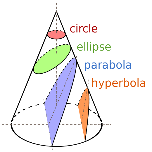
Fig. 49 Conic sections

Definition

A collection of points \((x,y)\in\mathbb{R}^2\), the sum of distances from which to two fixed points (termed foci) is constant, is an ellipse.

When the two foci coincide, the ellipse becomes a circle.

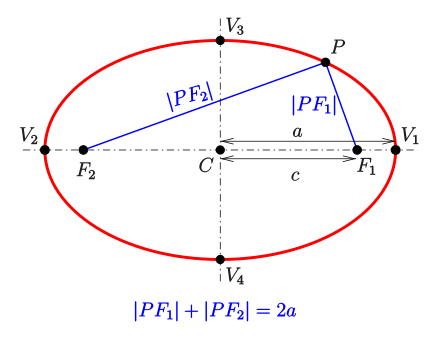
Canonical equation of an ellipse with parameters \(a\) and \(b\)

\[ \frac{x^2}{a^2}+\frac{y^2}{b^2} = 1 \]

When \(a=b\), the ellipse becomes a circle with radius \(a=b\).

Definition

Parabola is a collection of points \((x,y)\in\mathbb{R}^2\) laying at equal distances from a fixed point (focus) and a fixed line (directrix).

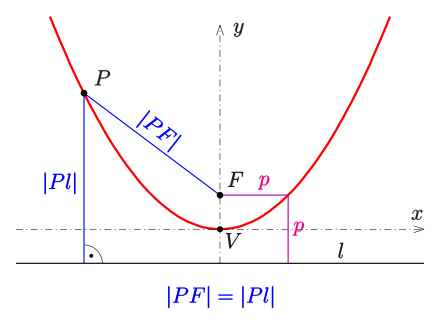
Parabola is a section of a cone by a plane parallel to another plane tangential to the conical surface.

Canonical equation of an ellipse with parameters \(a\) and \(b\)

\[ x^2 = 2py \]

Definition

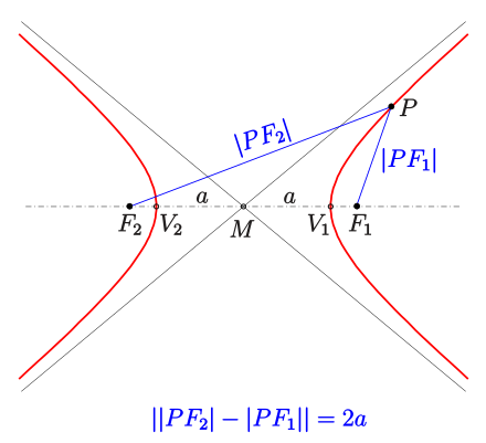
Hyperbola is a collection of points \((x,y)\in\mathbb{R}^2\), the difference of distances from which to two fixed points (termed foci) is constant.

Canonical equation of an ellipse with parameters \(a\) and \(b\)

\[ \frac{x^2}{a^2}-\frac{y^2}{b^2} = 1 \]

We typically encounter a hyperbola with the equation \(y=1/x\) or \(yx=1\), but it is easy to show that this is a special case with \(a=b\) after a change of basis with transformation matrix given by \(P=\begin{pmatrix}1/2&1/2\\1/2&-1/2\end{pmatrix}\)

Note

The highest power of \(x\) and \(y\) in the equation of a conic section is 2, hence the name quadratic curves.

Quadratic forms

Definition

Quadratic form in a function \(Q \colon \mathbb{R}^n \to \mathbb{R}\)

\[ Q(x) = \sum_{i=1}^n \sum_{j=1}^n a_{ij} x_i x_j \]

Note that we can assume that \(a_{ij} = a_{ji}\): indeed, if for some quadratic form \(\sum_{i=1}^n \sum_{j=1}^n c_{ij} x_i x_j\) symmetry does not hold, redefine

\[ a_{ij} = a_{ji} = \frac{c_{ij}+c_{ji}}{2} \]

then

\[\begin{split} \begin{array}{c} Q(x) = \sum_{i=1}^n \sum_{j=1}^n a_{ij} x_i x_j = \\ \begin{array}{cccccccc} a_{11} x_1 x_1 &+& a_{12} x_1 x_2 &+& \ldots &+& a_{1N} x_1 x_N & + \\ a_{21} x_2 x_1 &+& a_{22} x_2 x_2 &+& \ldots &+& a_{2N} x_2 x_N & + \\ \vdots & & \vdots & & \ddots & & \vdots & \\ a_{N1} x_N x_1 &+& a_{N2} x_N x_2 &+& \ldots &+& a_{NN} x_N x_N \end{array} = \\ \sum_{i=1}^n a_{ii} x_i^2 + 2 \sum_{i<j} a_{ij} x_i x_j = \\ = \sum_{i=1}^n c_{ii} x_i x_i + \sum_{i<j} (c_{ij}+c_{ji}) x_i x_j = \sum_{i=1}^n \sum_{j=1}^n c_{ij} x_i x_j \end{array} \end{split}\]

(See tutorial problem \(\gamma\).2)

Definition

Quadratic form \(Q \colon \mathbb{R}^n \to \mathbb{R}\) can be equivalently represented as a matrix product

\[ Q(x) = x^T A x \]

where \(x \in \mathbb{R}^n\) is a column vector, and \((n \times n)\) symmetric matrix \(A\) consists of elements \(\{a_{ij}\}\), \(i,j=1,\ldots,n\)

Example

\[ f: \mathbb{R}^3 \ni (x,y,z) \to x^2+3y^2-z^2-4xy+2yz \in \mathbb{R} \]

has a matrix representation with

\[\begin{split} A = \begin{pmatrix} 1 & -2 & 0 \\ -2 & 3 & 1 \\ 0 & 1 & -1 \end{pmatrix} \end{split}\]

Exercise: verify

Note

The degree of a quadratic form \(Q(x)\) which is a multivariate polynomial function is given by the sum of the powers of the variables, and for quadratic forms is not higher than 2, hence the name quadratic form. This implies that no term of the quadratic form may have a product of more than two variables!

Why are quadratic forms useful in the optimization course?

Look at the third term in the multivariate Taylor expansion of a function \(f(x) \colon \mathbb{R}^n \to \mathbb{R}\). It is a quadratic form!

We use quadratic forms for a local approximation of any function, and in second order conditions of optimization — later in the course.

Canonical form of quadratic forms

Definition

A canonical form of a quadratic form \(Q(x)\) is given by a sum of squares of the variables

\[ Q(x) = \sum_{i=1}^n a_i x_i^2 \]

Now it’s time to bring in all the machinery of matrix diagonalization!

Fact

Any quadratic form \(Q(x)\) can be brought to a canonical form by an orthogonal transformation \(P\).

\[ A = P^TDP, \quad Q(x) = x^T A x = \sum_{i=1}^n d_i (Px)_i^2 \]

where \(D\) is a diagonal matrix with elements \(d_i\) on the diagonal.

Proof

Because \(A\) is symmetric, the result follows from the fact that every symmetric matrix is diagonizable with an orthogonal matrix \(P\).

\[ Q(x) = x^T A x = x^T P^{-1} D P x = x^T P^T D P x = (Px)^T D (Px) = \sum_{i=1}^n d_i (Px)_i^2 \]

• When the eigenvalues of \(A\) are distinct, we also know that \(D\) contains them on the diagonal, and \(P\) is the matrix of normalized eigenvectors of \(A\).

• In practical tasks we will rely on having distinct eigenvalues and eigenvector diagonalization

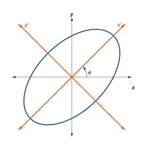
Fig. 50 Change of bases to convert the quadratic form to a canonical form

Definiteness of quadratic forms

The properties and shape of \(Q(x)\) depend on the configuration of matrix \(A\)

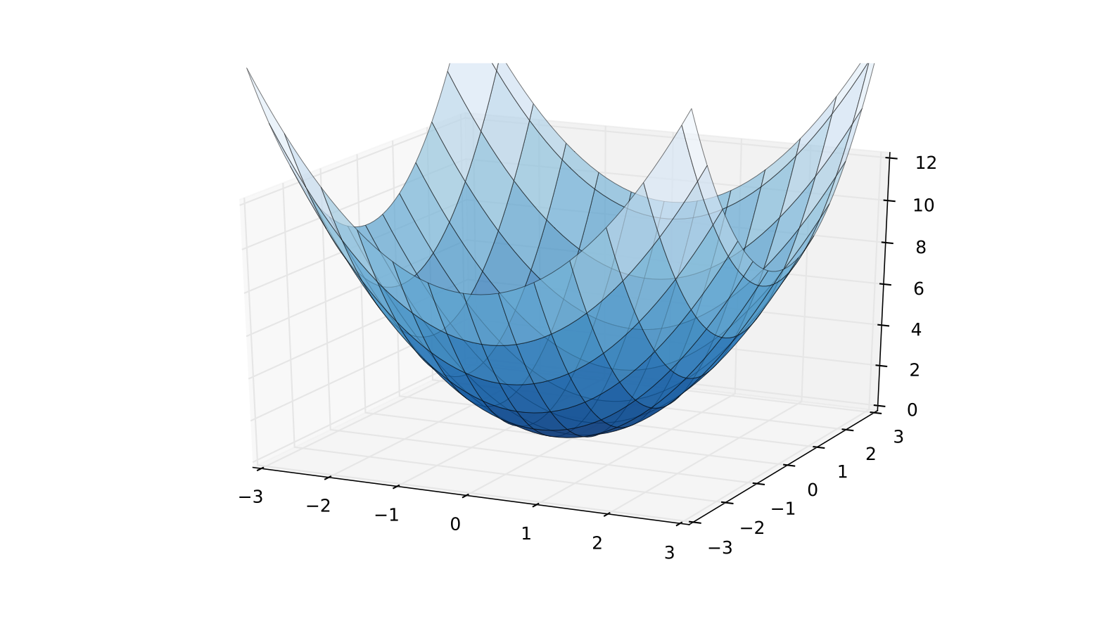
Fig. 51 A convex \(Q(x) = x' I x\)

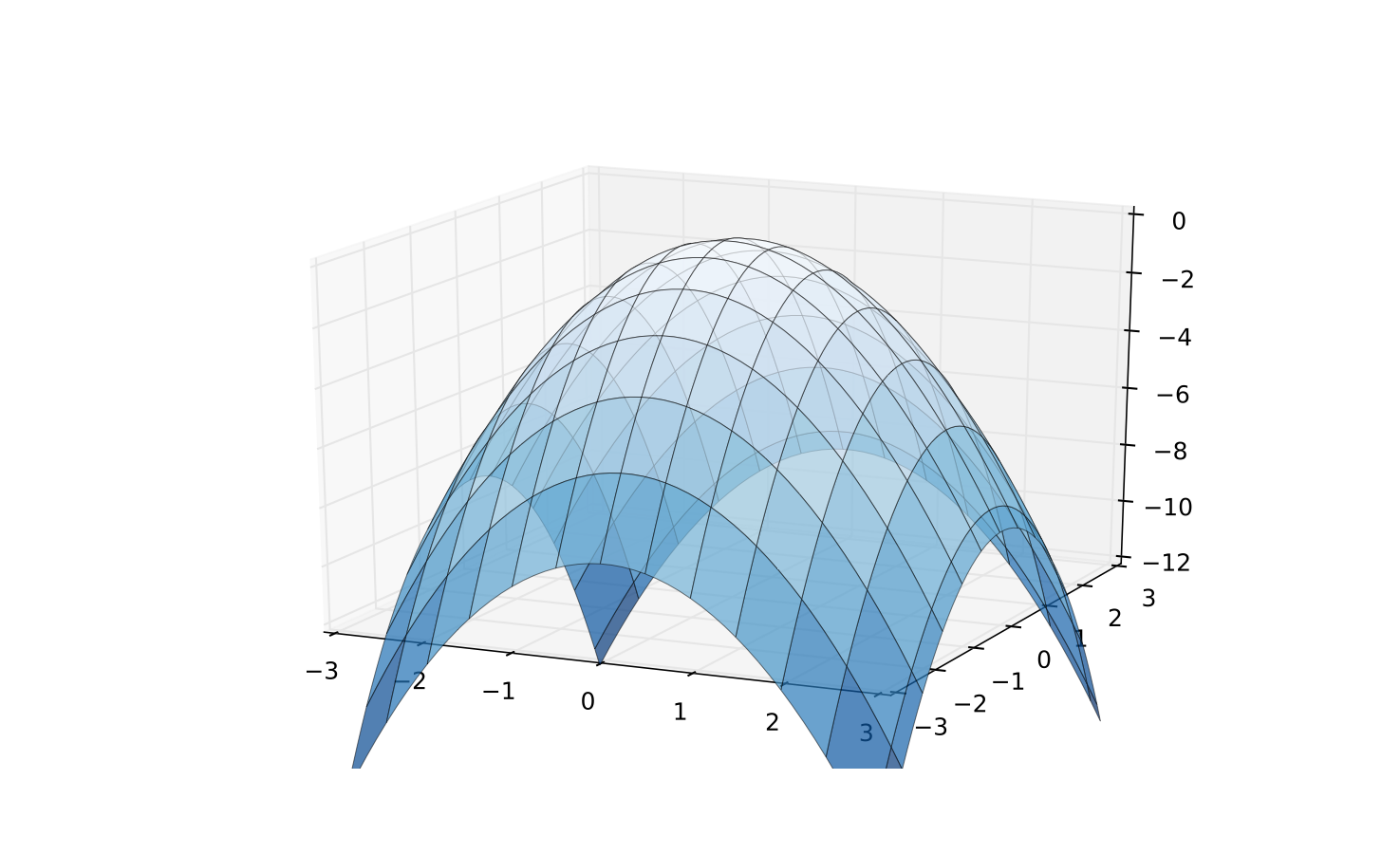
Fig. 52 A concave \(Q(x) = x'(-I)x\)

Definition

Quadratic form \(Q(x)\) is called positive definite if

\[ Q(x) = x^T A x >0 \text{ for all } x\ne 0 \]

Quadratic form \(Q(x)\) is called negative definite if

\[ Q(x) = x^T A x <0 \text{ for all } x\ne 0 \]

• the examples above show these cases

• note that because every quadratic form can be represented by a linear combination of squares, the characteristic properties are the signs of the coefficients in the canonical form!

Fact (Law of inertia)

The number of coefficients of a given sign in the canonical form of a quadratic form does not depend on the choice of the basis

• such robust characteristics are called invariants

• number of coefficients of a given sign is an invariant of the quadratic form called the index of the quadratic form

Definition

Positive and negative definite quadratic forms are called definite

Note that for some matrices it may be that

• for some \(x\): \(x^T A x < 0\)

• for some \(x\): \(x^T A x > 0\)

In this case \(A\) is called indefinite

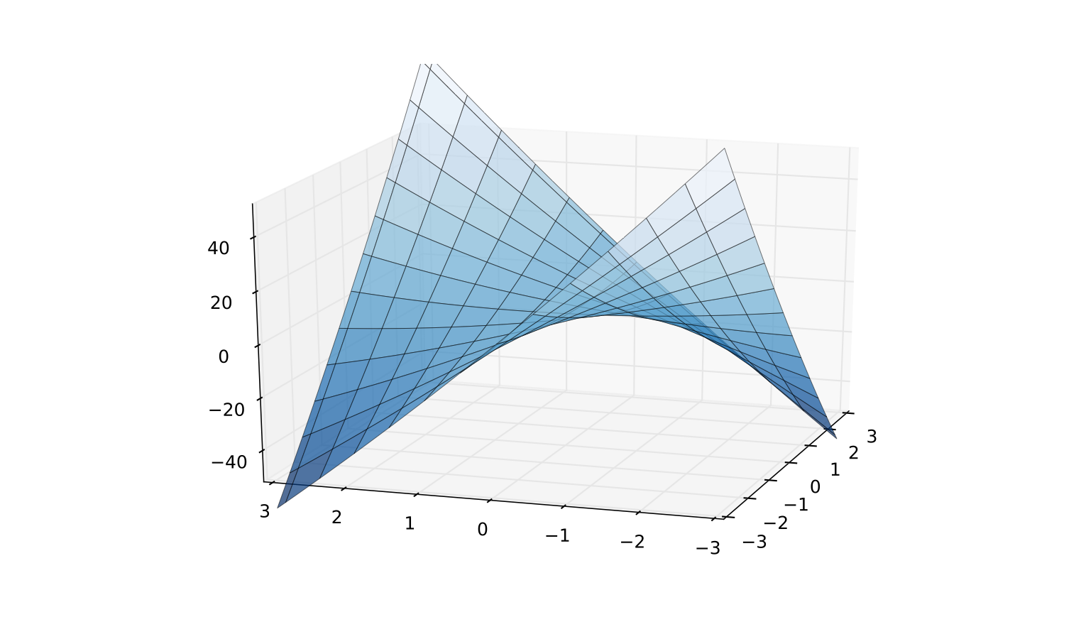
Fig. 53 Indefinite quadratic function \(Q(z) = x_1^2/2 + 8 x_1 x_2 + x_2^2/2\)

Example

\[\begin{split} \begin{array}{ll} Q(x) = x_1^2 + 2 x_2^2 + 1/2 x_3^2 & \text{positive definite} \\ Q(x) = x_1^2 - 2 x_2^2 & \text{indefinite} \\ Q(x) = x_1 x_2 & \text{indefinite} \\ Q(x) = 2 x_1 x_2 - x_1^2 - 4 x_2^2 = -(x_1-x_2)^2 - 3x_2^2 & \text{negative definite} \\ \end{array} \end{split}\]

• Note how immediately clear it is whether a quadratic form is positive or negative definite when it is written in the canonical form

Semi-definiteness of quadratic forms

• similar to weakly convex/concave functions

Definition

Quadratic form \(Q(x)\) is called non-negative definite (positive semi-definite) if

\[ Q(x) = x^T A x \geqslant 0 \text{ for all } x\ne 0 \]

Quadratic form \(Q(x)\) is called non-positive definite (negative semi-definite) if

\[ Q(x) = x^T A x \leqslant 0 \text{ for all } x\ne 0 \]

Example

\[\begin{split} \begin{array}{ll} Q(x) = x_1^2 + 2 x_2^2 & \text{positive semi-definite if } x \in \mathbb{R}^3\\ Q(x) = x_1^2 + 2x_1 x_2 + x_2^2 & \text{positive semi-definite} \\ \end{array} \end{split}\]

In the last example, the points \(t(1,-1)\) for any \(t \in \mathbb{R}\) yield \(Q(x) = 0\)

Because we know how to transform quadratic forms to the canonical form using eigenvalues, we can easily determine the definiteness of a quadratic form based on their signs

Fact (eigenvalues criterion)

A quadratic form \(Q(x)\) given by a symmetric matrix \(A\) which has distinct eigenvalues is

• positive definite \(\iff\) all eigenvalues are strictly positive

• negative definite \(\iff\) all eigenvalues are strictly negative

• nonnegative definite (positive semi-definite) \(\iff\) all eigenvalues are nonnegative

• nonpositive definite (negative semi-definite) \(\iff\) all eigenvalues are nonpositive

Proof

Follows immediately from the diagonalization of \(A\) and the canonical form of the quadratic form as sum of squares weighted by the eigenvalues.

\(\blacksquare\)

Example

\[ Q(x,y) = 8x^2 - 28xy + 29y^2 \]

\[\begin{split} A = \begin{pmatrix} 8 & -14 \\ -14 & 29 \end{pmatrix} \end{split}\]

Let’s diagonalize \(A\) by finding eigenvalues and eigenvectors

\[\begin{split} \left| \begin{array}{cc} 8-\lambda & -14 \\ -14 & -29-\lambda \end{array} \right| = (8-\lambda)(29-\lambda) - 14^2 = \lambda^2 - 37\lambda + 36 =0 \end{split}\]

Eigenvalues are \(\lambda_1 = 1\) and \(\lambda_2 = 36\)

Eigenvectors are \(v_1 = (2/\sqrt{5},1/\sqrt{5})\) and \(v_2 = (-1/\sqrt{5},2/\sqrt{5})\)

Transformation matrix (from eigen basis to current basis) is

\[\begin{split} P = \begin{pmatrix} 2/\sqrt{5} & -1/\sqrt{5} \\ 1/\sqrt{5} & 2/\sqrt{5} \end{pmatrix} \end{split}\]

and because \(A\) is symmetric, \(P\) is orthogonal, \(P^T = P^{-1}\). Denote the diagonal matrix \(D = \begin{pmatrix} 1 & 0 \\ 0 & 36 \end{pmatrix}\), thus we have \(A = P D P^T\).

Now with the change of variables \(\begin{pmatrix} u \\ v \end{pmatrix} = P^T \begin{pmatrix} x \\ y \end{pmatrix}\), that is \(u = \tfrac{2x+y}{\sqrt{5}}\) and \(v = \tfrac{2y-x}{\sqrt{5}}\) we can write the quadratic form as sum of squares of \(u\) and \(v\)

\[\begin{split} \tilde{Q}(u,v) = \begin{pmatrix} u \\ v \end{pmatrix}^T \begin{pmatrix} 1 & 0 \\ 0 & 36 \end{pmatrix} \begin{pmatrix} u \\ v \end{pmatrix} = u^2 + 36v^2 >0 \text{ for all } (u,v) \ne {\bf 0} \end{split}\]

Hense, \(Q(x)\) is a positive definite.

Fact

If quadratic form \(x^TAx\) is positive definite, and all eigenvalues of \(A\) are distinct, then \(\det(A) > 0\)

Proof

Positive definite \(\iff\) all eigenvalues are strictly positive \(\implies\) \(det(A)>0\) as the product of eigenvalues.

\(\blacksquare\)

• in particular, \(A\) is nonsingular

Silvester’s criterion

Diagonalization of the higher order matrices may be hard. We have an alternative for determining the definiteness of a quadratic form

Definition

Consider a \(n \times n\) matrix \(A\) and let \(0 < k \le n\).

The leading principal minor \(M_k\) of order \(k\) of \(A\) is the determinant of a matrix obtained from \(A\) by deleting its last \(n-k\) rows and columns.

Example

\[\begin{split} A = \left( \begin{array}{ccc} a_{11} & a_{12} & a_{13} \\ a_{21} & a_{22} & a_{23} \\ a_{31} & a_{32} & a_{33} \end{array} \right) \end{split}\]

The leading principal minors of oder \(k = 1,\dots,n\) of \(A\) are

\[\begin{split} \begin{array}{l} M_1 = \mathrm{det}(a_{11}) = a_{11} \\ M_2 = \mathrm{det}\left( \begin{array}{cc} a_{11} & a_{12} \\ a_{21} & a_{22} \end{array} \right) = a_{11}a_{22} - a_{12}a_{21} \\ M_3 = \mathrm{det}\left( \begin{array}{ccc} a_{11} & a_{12} & a_{13} \\ a_{21} & a_{22} & a_{23} \\ a_{31} & a_{32} & a_{33} \end{array} \right)\\ \vdots \\ M_n = \mathrm{det}(A) \end{array} \end{split}\]

Fact (definiteness)

Let \(A\) be an \((n \times n)\) symmetric square matrix. The corresponding quadratic form \(Q(x) = x^T A x\) is positive definite if and only if all leading principal minors of \(A\) are positive

\[ x^T A x > 0 \text{ for all } x \ne 0 \quad \iff \quad M_k > 0 \text{ for all } k=1,\ldots,n \]

Quadratic form \(Q(x) = x^T A x\) is negative definite if and only if the leading principal minors of \(A\) alternate in sign according to the following rule

\[ x^T A x < 0 \text{ for all } x \ne 0 \quad \iff \quad (-1)^k M_k >0 \text{ for all } k=1,\ldots,n \]

• the last condition can be restated as the leading principle minor \(M_k\) to have the same sign as \((-1)^k\)

• if \(A\) does not satisfy either of the conditions, it is indefinite or semi-definite

Silvester’s criterion for semi-definiteness

Silvester’s criterion for semi-definiteness is more involved

Definition

Consider a \(n \times n\) matrix \(A\) and let \(0 < k \le n\).

The principal minor \(P_k\) of order \(k\) of \(A\) is the determinant of a matrix obtained from \(A\) by deleting any of its \(n-k\) rows and columns with the same indexes.

• observe the difference from the leading principal minor

Example

\[\begin{split} A = \left( \begin{array}{ccc} a_{11} & a_{12} & a_{13} \\ a_{21} & a_{22} & a_{23} \\ a_{31} & a_{32} & a_{33} \end{array} \right) \end{split}\]

All the principal minors of oder \(k = 1,2,3\) of \(A\) are

\[\begin{split} \begin{array}{l} P^{a}_1 = \mathrm{det}(a_{11}) = a_{11} \\ P^{b}_2 = \mathrm{det}(a_{22}) = a_{22} \\ P^{c}_3 = \mathrm{det}(a_{33}) = a_{33} \\ P^{a}_2 = \mathrm{det}\left( \begin{array}{cc} a_{11} & a_{12} \\ a_{21} & a_{22} \end{array} \right) = a_{11}a_{22} - a_{12}a_{21} \\ P^{b}_2 = \mathrm{det}\left( \begin{array}{cc} a_{11} & a_{13} \\ a_{31} & a_{33} \end{array} \right) = a_{11}a_{33} - a_{13}a_{31} \\ P^{c}_2 = \mathrm{det}\left( \begin{array}{cc} a_{22} & a_{23} \\ a_{32} & a_{33} \end{array} \right) = a_{22}a_{33} - a_{23}a_{32} \\ P_3 = \mathrm{det}\left( \begin{array}{ccc} a_{11} & a_{12} & a_{13} \\ a_{21} & a_{22} & a_{23} \\ a_{31} & a_{32} & a_{33} \end{array} \right) \end{array} \end{split}\]

Fact (semi-definiteness)

Let \(A\) be an \((n \times n)\) symmetric square matrix. The corresponding quadratic form \(Q(x) = x^T A x\) is positive semi-definite if and only if all principal minors of \(A\) are non-negative.

\[ x^T A x \geqslant 0 \text{ for all } x \ne 0 \quad \iff \quad \forall P_k: P_k \geqslant 0 \text{ for all } k=1,\ldots,n \]

Quadratic form \(Q(x) = x^T A x\) is negative semi-definite if and only if all principal minors of oder \(k\) of \(A\) are zero or have the same sign as \((-1)^k\)

\[ x^T A x \leqslant 0 \text{ for all } x \ne 0 \quad \iff \quad \forall P_k : (-1)^k P_k \geqslant 0 \text{ for all } k=1,\ldots,n \]

Example

\[\begin{split} A = \left( \begin{array}{ccc} 4 & 0 & 1 \\ 0 & 2 & 0 \\ 1 & 0 & 1 \end{array} \right) \end{split}\]

The leading principal minors of \(A\) are

\[\begin{split} \begin{array}{l} M_1 = \mathrm{det}(4) = 4 \\ M_2 = \mathrm{det}\left( \begin{array}{cc} 4 & 0 \\ 0 & 2 \end{array} \right) = 4 \cdot 2 - 0 = 8 \\ M_3 = \mathrm{det}\left( \begin{array}{ccc} 4 & 0 & 1 \\ 0 & 2 & 0 \\ 1 & 0 & 1 \end{array} \right) = 4\cdot 2 - 2 = 6 \end{array} \end{split}\]

All leading principal minors are positive, hence \(x^TAx\) is positive definite.

Let’s verify the result by computing the eigenvalues of \(A\).

\[\begin{split} \det\left( \begin{array}{ccc} 4-\lambda & 0 & 1 \\ 0 & 2-\lambda & 0 \\ 1 & 0 & 1-\lambda \end{array} \right) = (4-\lambda)(2-\lambda)(1-\lambda) - (2-\lambda) \end{split}\]

The eigenvalues of \(A\) are \(\{2,\tfrac{5+\sqrt{13}}{2},\tfrac{5-\sqrt{13}}{2}\}\), that is all positive, and therefore the same conclusion is reached by the eigenvalues criterion.

Example

\[\begin{split} B = \left( \begin{array}{ccc} 3 & 0 & -3 \\ 0 & -1 & 1 \\ -3 & 1 & 2 \end{array} \right) \end{split}\]

The leading principal minors of \(B\) are

\[\begin{split} \begin{array}{l} M_1 = \mathrm{det}(3) = 3 \\ M_2 = \mathrm{det}\left( \begin{array}{cc} 3 & 0 \\ 0 & -1 \end{array} \right) = 3 (-1) - 0 = -3 \\ M_3 = \mathrm{det}\left( \begin{array}{ccc} 3 & 0 & -3 \\ 0 & -1 & 1 \\ -3 & 1 & 2 \end{array} \right) = -6 + 9 - 3 = 0 \end{array} \end{split}\]

The leading principal minors do not match neither the rule for positive definiteness (all positive) nor the rule for negative definiteness (alternating signs). But the rule for the negative semi-definiteness may still be satisfied, hence let’s examine the rest of principal minors.

The other (non-leading) principal minors of order \(k=1\) of \(B\) are

\[\begin{split} \begin{array}{l} M^2_1 = \mathrm{det}(-1) = -1 \\ M^3_1 = \mathrm{det}(2) = 2 \\ \end{array} \end{split}\]

and it is clear that the rule for negative semi-definiteness is not satisfied: principle minors of oder 1 differ in signs.

Thus, \(x^TBx\) is indefinite.

Let’s verify this conclusion using the eigenvalues criterion.

\[\begin{split} \det\left( \begin{array}{ccc} 3-\lambda & 0 & -3 \\ 0 & -1-\lambda & 1 \\ -3 & 1 & 2-\lambda \end{array} \right) = -(3-\lambda)(\lambda+1)(2-\lambda) + 9 (\lambda+1) - (3-\lambda) = -\lambda (\lambda^2 -4\lambda -7) \end{split}\]

The eigenvalues of \(A\) are \(\{0,2+\sqrt{11},2-\sqrt{11}\}\), and since the latter is negative they differ is sing. Therefore \(B\) is indefinite also by the eigenvalues criterion.

Show code cell content Hide code cell content

import numpy as np
import matplotlib.pyplot as plt
from mpl_toolkits.mplot3d import Axes3D
from myst_nb import glue

A = np.array([[-1,-np.sqrt(2)],[-np.sqrt(2),-2]])
f = lambda x: x@A@x
x = y = np.linspace(-5.0, 5.0, 100)
X, Y = np.meshgrid(x, y)
zs = np.array([f((x,y)) for x,y in zip(np.ravel(X), np.ravel(Y))])
Z = zs.reshape(X.shape)

fig = plt.figure(dpi=160)
ax3 = fig.add_subplot(111, projection='3d')
ax3.plot_wireframe(X, Y, Z, 
            rstride=2, 
            cstride=2,
            alpha=0.7,
            linewidth=0.25)
f0 = f(np.zeros((2)))+0.1
ax3.plot([-5,5],[5/np.sqrt(2),-5/np.sqrt(2)],[f0,f0],color='black',linewidth=0.5)
plt.setp(ax3,xticks=[],yticks=[],zticks=[])
glue("fig_example", fig, display=False)

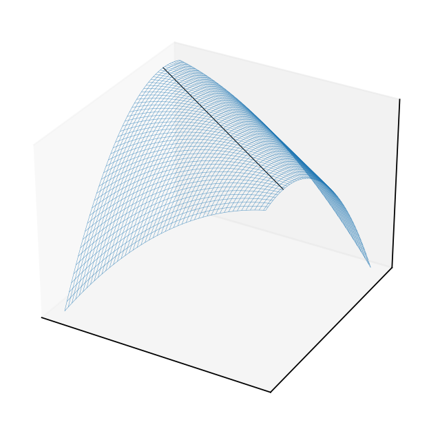
Example

\[\begin{split} C = \left( \begin{array}{cc} -1 & -\sqrt{2} \\ -\sqrt{2} & -2 \end{array} \right) \end{split}\]

The leading principal minors of \(C\) are

\[\begin{split} \begin{array}{l} M_1 = \mathrm{det}(-1) = -1 \\ M_2 = \mathrm{det}\left( \begin{array}{cc} -1 & -\sqrt{2} \\ -\sqrt{2} & -2 \end{array} \right) = 2 - 2 = 0 \end{array} \end{split}\]

The leading principal minors do not match neither the rule for positive definiteness (all positive) nor the rule for negative definiteness (alternating signs). But the rule for the negative semi-definiteness may still be satisfied, hence let’s examine the rest of principal minors, namely one more principle minor of order 1:

\[ M^2_1 = \mathrm{det}(-2) = -2 \]

Ok, the pattern for negative semi-definiteness is satisfied!

Thus, \(x^TCx\) is negative semi-definite.

The plot of the quadratic form \(x^TCx\) is below. Note the line of zero values of the quadratic form attained at many different non-zero points \((-p,p/\sqrt{2})\), where \(p \in \mathbb{R}\).

Fig. 54 The shape of the quadratic form in the example