Announcements & Reminders

1. Quizzes

• All grading is done for Quiz 1

• Quiz 2 is next Monday, March 25 8:00 to 23:59, same setup

2. The midterm is scheduled at 18:30 to 19:45 (1 hour + 15 min reading time) on Monday, April 15 in Melville Hall

📖 Multivariate calculus

⏱ | words

Today we continue to get comfortable with the multidimensional space of real numbers \(\mathbb{R}^N\)

Main goal: learn and practice multidimensional differentiation

But first

• Refresh definition of derivative and differentiability

Revision of univariate differentiation

Derivatives

Definition

Let \(f \colon X \to \mathbb{R}\)

Let \(H\) be the set of all convergent sequences \(\{h_n\}\) such that \(h_n \ne 0\) and \(h_n \to 0\)

If there exists a constant \(f'(x)\) such that

\[ \frac{f(x + h_n) - f(x)}{h_n} \to f'(x) \]

for every \(\{h_n\} \in H\), then

• \(f\) is said to be differentiable at \(x\)

• \(f'(x)\) is called the derivative of \(f\) at \(x\)

We will use the following notation for derivative interchangeably

\[f'(x) \quad \frac{df}{dx} \quad \frac{d}{dx}f(x)\]

Definition

A function \(f \colon X \to \mathbb{R}\) is called differentiable (on \(X\)) if it is differentiable in all points of \(X\)

Example

Let \(f \colon \mathbb{R} \to \mathbb{R}\) be defined by \(f(x) = x^2\)

Fix any \(x \in \mathbb{R}\) and any \(h_n \to 0\) with \(n \to \infty\)

We have

\[ \frac{f(x + h_n) - f(x)}{h_n} = \frac{(x + h_n)^2 - x^2}{h_n} = \]

\[ = \frac{x^2 + 2xh_n + h_n^2 - x^2}{h_n} = 2x + h_n \]

\[ \text{therefore } f'(x) = \lim_{n \to \infty} (2x + h_n) = 2x + \lim_{n \to \infty} h_n = 2x \]

Example

Let \(f \colon \mathbb{R} \to \mathbb{R}\) be defined by \(f(x) = |x|\)

This function is not differentiable at \(x=0\)

Indeed, if \(h_n = 1/n\), then

\[ \frac{f(0 + h_n) - f(0)}{h_n} = \frac{|0 + 1/n| - |0|}{1/n} \to 1 \]

On the other hand, if \(h_n = -1/n\), then

\[ \frac{f(0 + h_n) - f(0)}{h_n} = \frac{|0 - 1/n| - |0|}{-1/n} \to -1 \]

Therefore the definition of the derivative is not satisfied

Heine and Cauchy definitions of the limit for functions

As a side note, let’s mention that there are two ways to define the limit of a function \(f\).

In the last lecture when talking about continuity and just above in the definition of the derivative we implicitly used the definition of function limit defined through limit of sequences, due to Eduard Heine

Definition (Limit of a function due to Heine)

Given the function \(f: A \subset \mathbb{R}^N \to \mathbb{R}\), \(a \in \mathbb{R}\) is a limit of \(f(x)\) as \(x \to x_0 \in A\) if

\[\forall \{x_n\} \in A \colon \lim_{n \to \infty} x_n = x_0 \in A \quad \implies \quad f(x_n) \to a \]

The alternative definition of the limit is due to Augustin-Louis Cauchy, also known as \(\epsilon\)-\(\delta\) definition

Definition (Limit of a function due to Cauchy)

Given the function \(f: A \subset \mathbb{R}^N \to \mathbb{R}\), \(a \in \mathbb{R}\) is a limit of \(f(x)\) as \(x \to x_0 \in A\) if

\[\forall \, \epsilon > 0, \; \exists \, \delta >0 \; \text{ such that } 0 < |x − x_0| < \delta \implies |f(x) − a| < \epsilon\]

• note the similarity to the definition of the sequence

• note that in the \(\epsilon\)-ball around \(x_0\) the point \(x_0\) is excluded

Fig. 45 \(\lim_{x \to x_0} f(x) = L\) under the Cauchy definition

Fact

Cauchy and Heine definitions of the function limit are equivalent

Therefore we can use the same notation of the definition of the limit of a function

\[\lim_{x \to x_0} f(x) = a \quad \text{or} \quad f(x) \to a \; \text{as} \; x \to x_0\]

Differentiation rules

Fact

For functions \(f(x)\), \(g(x)\) and \(h(x)\), and constant \(c\), we have

• Scalar Multiplication Rule

\[f(x) = c g(x) \quad\implies\quad f^{\prime}(x)=c g^{\prime}(x)\]

• Summation Rule:

\[f(x) = g(x) + h(x) \quad\implies\quad f^{\prime}(x)=g^{\prime}(x)+h^{\prime}(x)\]

• Product Rule:

\[f(x) = g(x)h(x) \quad\implies\quad f^{\prime}(x)=g^{\prime}(x) h(x)+h^{\prime}(x) g(x)\]

• Quotient Rule:

\[f(x) = g(x)/h(x), \; h(x)\ne 0 \quad\implies\quad f^{\prime}(x)=\frac{g^{\prime}(x) h(x)-h^{\prime}(x) g(x)}{[h(x)]^{2}}\]

• Chain Rule:

\[f(x) = (g \circ h)(x) = g\big( h(x) \big) \quad\implies\quad f^{\prime}(x)=g^{\prime}(h(x)) h^{\prime}(x)\]

• The Inverse Function Rule:

\[y = f(x), \; g(y) = f^{-1}(y) \; \text{is well defined} \quad\implies\quad g^{\prime}(y) = \frac{1}{f^{\prime}\big( f^{-1}(y) \big)}\]

Differentiability and continuity

Just a reminder: by definition a function \(f: X \to \mathbb{R}\) is continuous in \(a\) if \(f(x) \to f(a)\) as \(x \to a\)

Fact

A differentiable function \(f \colon X \to \mathbb{R}\) is continuous on \(X\).

Converse is not true in general.

\[\begin{split}\text{Differentiability} \quad \begin{array}{c} \Longrightarrow \\ \not \Longleftarrow \end{array} \quad \text{Continuity}\end{split}\]

Proof

Consider a function \(f: X \longrightarrow \mathbb{R}\) where \(X \subseteq \mathbb{R}\). Suppose that

\[ \lim _{h \rightarrow 0}\left(\frac{f(a+h)-f(a)}{h}\right) \]

exists.

We want to show that this implies that \(f(x)\) is continuous at the point \(a \in X\). The following proof of this proposition is drawn from [Ayres Jr and Mendelson, 2013] (Chapter 8, Solved Problem 2).

First, note that

\[\begin{split} \begin{gathered} \lim _{h \rightarrow 0}(f(a+h)-f(a))=\lim _{h \rightarrow 0}\left\{\left(\frac{h}{h}\right)(f(a+h)-f(a))\right\} \\ =\lim _{h \rightarrow 0}\left\{h\left(\frac{f(a+h)-f(a)}{h}\right)\right\} \\ =\lim _{h \rightarrow 0}(h) \lim _{h \rightarrow 0}\left(\frac{f(a+h)-f(a)}{h}\right) \\ =(0)\left(\lim _{h \rightarrow 0}\left(\frac{f(a+h)-f(a)}{h}\right)\right) \\ =0 . \end{gathered} \end{split}\]

Thus we have

\[ \lim _{h \rightarrow 0}(f(a+h)-f(a))=0 . \]

Now note that

\[\begin{split} \begin{gathered} \lim _{h \rightarrow 0}(f(a+h)-f(a))=\lim _{h \rightarrow 0} f(a+h)-\lim _{h \rightarrow 0} f(a) \\ =\left(\lim _{h \rightarrow 0} f(a+h)\right)-f(a) \end{gathered} \end{split}\]

Upon combining these two results, we obtain

\[ \left(\lim _{h \rightarrow 0} f(a+h)\right)-f(a)=0 \Longleftrightarrow \lim _{h \rightarrow 0} f(a+h)=f(a) . \]

Finally, note that

\[ \lim _{x \rightarrow a} f(x)=\lim _{h \rightarrow 0} f(a+h) . \]

Thus we have

\[ \lim _{x \rightarrow a} f(x)=f(a) \]

This means that \(f(x)\) is continuous at the point \(x=a\).

---

Consider the function

\[\begin{split} f(x)=\left\{\begin{array}{cc} 2 x & \text { if } x \leqslant 1 \\ \frac{1}{2} x+\frac{3}{2} & \text { if } x \geq 1 \end{array}\right. \end{split}\]

(There is no problem with this double definition at the point \(x=1\) because the two parts of the function are equal at that point.)

This function is continuous at \(x=1\) because

\[ \lim _{x \rightarrow 1} 2 x=2=\lim _{x \rightarrow 1}\left(\frac{1}{2} x+\frac{3}{2}\right) \]

and

\[ f(1)=2 \]

However, this function is not differentiable at \(x=1\) because

\[ \lim _{h \uparrow 1} \frac{f(1+h)-f(1)}{h}=2 \]

and

\[ \lim _{h \downarrow 1} \frac{f(1+h)-f(1)}{h}=\frac{1}{2} \]

Since

\[ \lim _{h \uparrow 1} \frac{f(1+h)-f(1)}{h} \neq \lim _{h \downarrow 1} \frac{f(1+h)-f(1)}{h} \]

we know that

\[ \lim _{h \rightarrow 1} \frac{f(1+h)-f(1)}{h} \]

does not exist.

\(\blacksquare\)

Higher order derivatives

Consider a derivative \(f'(x)\) of a function \(f(x)\) as a new function \(g(x)\). We can then take the derivative of \(g(x)\) to obtain a second order derivative of \(f(x)\), denoted by \(f''(x)\).

Definition

Let \(f \colon X \to \mathbb{R}\) and let \(x \in (a, b)\)

A second order derivative of \(f\) at \(x\) denoted \(f''(x)\) or \(\frac{d^2 f}{dxdx}\) is the (first order) derivative of the function \(f'(x)\), if it exists

More generally, the \(k\)-th order derivative of \(f\) at \(x\) denoted \(f^{(m)}(x)\) or \(\frac{d^k f}{dx \dots dx}\) is the derivative of function \(\frac{d^{k-1} f}{dx \dots dx}\), if it exists

Definition

The function \(f: X \to \mathbb{R}\) is said to be of differentiability class \(C^m\) if derivatives \(f'\), \(f''\), \(\dots\), \(f^{(m)}\) exist and are continuous on \(X\)

Taylor series

Fact

Consider \(f: X \to \mathbb{R}\) and let \(f\) to be a \(C^m\) function. Assume also that \(f^{(m+1)}\) exists, although may not necessarily be continuous.

For any \(x,a \in X\) there is such \(z\) between \(a\) and \(x\) that

\[\begin{split}\begin{array}{rl} f(x) =& f(a) + f'(a)(x-a) + \dots + \frac{f^{(m)}(a)}{m!}(x-a)^m + R_m(x) =\\ =& f(a) + \sum_{k=1}^m \frac{f^{(k)}(a)}{k!}(x-a)^k + R_m(x), \end{array}\end{split}\]

where the remainder is given by

\[R_m(x) = \frac{f^{(m+1)}(z)(x-a)^{m+1}}{(m+1)!} = o\big((x-a)^m\big)\]

Definition

Little-o notation is used to describe functions that approach zero faster than a given function

\[f(x) = o\big(g(x)\big) \; \text{as} \; x \to a \quad \iff \quad \lim_{x \to a} \frac{f(x)}{g(x)} = 0\]

Loosely speaking, if \(f \colon \mathbb{R} \to \mathbb{R}\) is suitably differentiable at \(a\), then

\[ f(x) \approx f(a) + f'(a)(x-a) \]

for \(x\) very close to \(a\),

\[ f(x) \approx f(a) + f'(a)(x-a) + \frac{f''(a)}{2!}(x-a)^2 \]

on a slightly wider interval, etc.

These are the 1st and 2nd order Taylor series approximations to \(f\) at \(a\) respectively

As the order goes higher we get better approximation

Fig. 46 4th order Taylor series for \(f(x) = \sin(x)/x\) at 0

Fig. 47 6th order Taylor series for \(f(x) = \sin(x)/x\) at 0

Fig. 48 8th order Taylor series for \(f(x) = \sin(x)/x\) at 0

Fig. 49 10th order Taylor series for \(f(x) = \sin(x)/x\) at 0

Multivariate differentiation

Functions from \(\mathbb{R}^N\) to \(\mathbb{R}\)

Extending the one-dimensional definition of derivative to multi-variate case is tricky!

With multiple variables, we have to decide which one to increment with the elements of the sequence \(\{h_n\}\)

We need a \(i\)-th unit vector of the form \((0, \dots, 0, 1, 0, \dots, 0)\) where \(1\) is in the \(i\)-th position to choose one particular variable

Definition

Let \(f \colon A \to \mathbb{R}\) and let \(x \in A \subset \mathbb{R}^N\). Denote \(e_i\) the \(i\)-th unit vector in \(\mathbb{R}^N\), i.e. \(e_i = (0, \dots, 0, 1, 0, \dots, 0)\) where \(1\) is in the \(i\)-th position.

If there exists a constant \(a \in \mathbb{R}\) such that

\[ \frac{f(x + h_n e_i) - f(x)}{h_n} \to a \]

for every sequence \(\{h_n\}\), \(h_n \in \mathbb{R}\), such that \(h_n \ne 0\) and \(h_n \to 0\) as \(n \to \infty\), then \(a\) is called a partial derivative of \(f\) with respect to \(x_i\) at \(x\), and is denoted

\[ f'_i(x) \quad \text{or} \quad \frac{\partial f}{\partial x_i}(x) \]

• Note the slight difference in notation \(\frac{d f}{d x}(x)\) of univariate derivative and \(\frac{\partial f}{\partial x_i}(x)\) of partial derivative

• Partial derivatives behave just like regular derivatives of the univariate functions, assuming all variables except one are treated as constants

• Usual rules of differentiation apply

Example

\[\begin{split} f \colon \left( \begin{array}{c} x_1 \\ x_2 \\ x_3 \end{array} \right) \mapsto x_1^2 + x_2 x_3 \end{split}\]

Partial derivatives are

\[ \frac{\partial f}{\partial x_1} = 2 x_1, \; \frac{\partial f}{\partial x_2} = x_3, \; \frac{\partial f}{\partial x_3} = x_2 \]

However, the partial derivatives do not get it there all the way:

• full analogue of the multivariate derivative to the univariate one should include all sequences converging to zero in the \(\mathbb{R}^N\) space?

• what is the analogue of differentiability in the multivariate case, with the same implication to the continuety?

Definition

Let

• \(A \subset \mathbb{R}^N\) be an open set in \(N\)-dimensional space

• \(f \colon A \to \mathbb{R}\) be multivariate function

• \(x \in A\), and so \(\exists \epsilon \colon B_{\epsilon}(x) \subset A\)

Then if there exists a vector \(g \in \mathbb{R}^N\) such that

\[ \frac{f(x + h_n) - f(x) - g \cdot h_n}{\|h_n\|} \to 0 \]

for all converging to zero sequences \(\{h_n\}\), \(h_n \in B_{\epsilon}(0) \setminus \{0\}\), \(h_n \to 0\), then

• \(f\) is said to be differentiable at \(x\)

• vector \(g\) is called the gradient of \(f\) at \(x\), and is denoted by \(\nabla f(x)\) or simply \(f'(x)\)

• note the dot product of \(g\) and \(h_n\) in the definition

• the gradient is a vector of partial derivatives

Fact

If a function \(f \colon \mathbb{R}^N \to \mathbb{R}\) is differentiable at \(x\), then all partial derivatives at \(x\) exist and the gradient is given by

\[ \nabla f(x) = \left( \frac{\partial f}{\partial x_1}(x), \dots, \frac{\partial f}{\partial x_N}(x) \right) \]

Proof

The idea of the proof: consider all converging sequences in \(\mathbb{R}^N\) and corresponding set of sequences in each dimension, component-wise.

Example

Continuing the previous example, the gradient is

\[ \nabla f(x) = \left( 2x_1, \, x_3, \, x_2 \right) \]

Now, evaluating at a particular points (bold \({\bf 1}\) and \({\bf 0}\) denotes unit vector and zero vector in \mathbb{R}^3)

\[ \nabla f({\bf 0}) = \left( 0, \, 0, \, 0 \right) \]

\[ \nabla f({\bf 1}) = \left( 2, \, 1, \, 1 \right) \]

\[ \nabla f((1,2,3)^T) = \left( 2, \, 3, \, 2 \right) \]

Fact

Sufficient conditions for differentiability of a function \(f \colon \mathbb{R}^N \to \mathbb{R}\) at \(x\) are that all partial derivatives exist and are continuous in \(x\)

Proof

The idea of the proof: consider all converging sequences in \(\mathbb{R}^N\) as composed component-wise from the converging sequences in each dimension, and verify that due to continuity, the vector of partial derivatives forms the vector \(g\) required by the definition of differentiability.

Directional derivatives

To understand the role of the gradient of \(\mathbb{R}^N \to \mathbb{R}\) function, we need to introduce the concept of the directional derivative

Direction in \(\mathbb{R}^N\) can be given by any vector, after all vector has

• absolute value (length)

• direction But we should focus on the unit vectors, i.e. vectors of length 1

Definition

Let

• \(A \subset \mathbb{R}^N\) be an open set in \(N\)-dimensional space

• \(f \colon A \to \mathbb{R}\) be multivariate function

• \(x \in A\), and so \(\exists \epsilon \colon B_{\epsilon}(x) \subset A\)

• \(v \in \mathbb{R}^N\) is a unit vector, i.e. \(\|v\| = 1\)

Then if there exists a constant \(D_v f(x) \in \mathbb{R}\) such that

\[\lim_{h \to 0} \frac{f(x + hv) - f(x)}{h} = D_v f(x)\]

then it is called a directional derivative of \(f\) at \(x\) in the direction of \(v\)

• note that the step size \(h\) here is scalar

• the directional derivative is a scalar as well

• the whole expression \(\frac{f(x + hv) - f(x)}{h}\) can be thought of a univariate function of \(h\)

• the directional derivative is a simple (univariate) derivative of this function

Example

\[\begin{split} f \colon \left( \begin{array}{c} x_1 \\ x_2 \\ x_3 \end{array} \right) \mapsto x_1^2 + x_2 x_3 \end{split}\]

Let \(v = (\frac{1}{\sqrt{2}},\frac{1}{\sqrt{2}},0)\), that is we are interested in the derivative along the \(45^\circ\) line in the \(x\)-\(y\) plane. Note that \(\|v\|=1\).

After substitution of \(x+hv\) into \(f\), we get the function

\[\begin{split} g(x,h) = f(x+hv) = f\left( \begin{array}{c}x_1+h/\sqrt{2}\\x_2+h/\sqrt{2}\\x_3\end{array} \right) = (x_1+h/\sqrt{2})^2 + (x_2+h/\sqrt{2}) x_3 \end{split}\]

Differentiating \(g(x,h)\) with respect to \(h\) gives

\[ \frac{\partial g}{\partial h}(x,h) = \sqrt{2}(x_1+h/\sqrt{2}) + x_3/\sqrt{2} \]

Finally, because we are interested in the derivative at the point \(x\) corresponding to \(h=0\), we have

\[ D_v f(x) = \left. \frac{\partial g}{\partial h}(x,h) \right|_{h=0} = \sqrt{2}x_1 + \frac{x_3}{\sqrt{2}} \]

Fact

Directional derivative of a differentiable function \(f \colon \mathbb{R}^N \to \mathbb{R}\) at \(x\) in given by

\[D_v f(x) = \nabla f(x) \cdot v = \sum_{i=1}^N \frac{\partial f}{\partial x_i}(x) v_i\]

Proof

Main idea: carefully convert the limit from the definition of differentiability of \(f\) to the univariate limit in the definition of the directional derivative. The latter happens to equal teh dot product of the gradient and the direction vector.

Example

Continuing the previous example, we have \(v = (\frac{1}{\sqrt{2}},\frac{1}{\sqrt{2}},0)\) and

\[ \frac{\partial f}{\partial x_1} = 2 x_1, \; \frac{\partial f}{\partial x_2} = x_3, \; \frac{\partial f}{\partial x_3} = x_2 \]

Therefore, applying the formula \(D_v f(x) = \nabla f(x) \cdot v\) we immediately have

\[ D_v f(x) = \sqrt{2} x_1 + \frac{x_3}{\sqrt{2}} \]

Fact

The direction of the fastest ascent of a differentiable function \(f \colon \mathbb{R}^N \to \mathbb{R}\) at \(x\) is given by the direction of its gradient \(\nabla f(x)\).

Proof

First, Cauchy–Bunyakovsky–Schwarz inequality for a Euclidean space \(\mathbb{R}^N\) states that for any two vectors \(u, v \in \mathbb{R}^N\) we have

\[|u \cdot v| \leqslant \|u\| \|v\|\]

where “\(\cdot\)” is dot product and \(\|x\| = \sqrt{x \cdot x}\) is the standard Euclidean norm.

Consider the case when at least one element of \(\nabla f(x)\) is positive, otherwise \(D_v f(x) = 0\) implying that the function does not increase in any direction.

For any unit direction vector \(v\) (in the same general direction as \(\nabla f(x)\) so that \(\nabla f(x) \cdot v >0\)), we have

\[D_v f(x) = \nabla f(x) \cdot v \leqslant \|\nabla f(x)\| \|v\| = \|\nabla f(x)\|\]

The inequality is due to Cauchy–Bunyakovsky–Schwarz.

Now consider \(v = \frac{\nabla f(x)}{\|\nabla f(x)\|}\). For this direction vector we have

\[D_v f(x) = \nabla f(x) \cdot \frac{\nabla f(x)}{\|\nabla f(x)\|} = \frac{\nabla f(x) \cdot \nabla f(x)}{\|\nabla f(x)\|} = \frac{(\|\nabla f(x)\|)^2}{\|\nabla f(x)\|} = \|\nabla f(x)\|\]

Thus, the upper bound on \(D_v f(x)\) is achieved when vector \(v\) has the same direction as gradient vector \(\nabla f(x)\). \(\blacksquare\)

• Steepest descent algorithm uses the opposite direction of the gradient

• Stochastic steepest descent algorithm uses the same idea (ML and AI applications!)

Functions from \(\mathbb{R}^N\) to \(\mathbb{R}^K\)

Let’s now consider more complex case: functions from multi-dimensional space to multi-dimensional space

Definition

The vector-valued function \(f \colon \mathbb{R}^N \to \mathbb{R}^K\) is a tuple of \(K\) functions \(f_j \colon \mathbb{R}^N \to \mathbb{R}\), \(j \in \{1, \dots, K\}\)

We shall typically assume that the vector-valued functions return a column-vector

Definition

Let

• \(A \subset \mathbb{R}^N\) be an open set in \(N\)-dimensional space.

• \(f \colon A \to \mathbb{R}^K\) be a \(K\) dimensional vector function

• \(x \in A\), and so \(\exists \epsilon \colon B_{\epsilon}(x) \subset A\)

Then if there exists a \((K \times N)\) matrix \(J\) such that

\[ \frac{\|f(x + h_n) - f(x) - J h_n\|}{\|h_n\|} \to 0 \]

for all converging to zero sequences \(\{h_n\}\), \(h_n \in B_{\epsilon}(0) \setminus \{0\}\), \(h_n \to 0\), then

• \(f\) is said to be differentiable at \(x\)

• matrix \(J\) is called the total derivative (or Jacobian matrix) of \(f\) at \(x\), and is denoted by \(Df(x)\) or simply \(f'(x)\)

• in this definition \(h_n\) is also a converging to zero sequence in \(\mathbb{R}^N\)

• the different is that in the numerator we have to use the norm to measure the distance in the \(\mathbb{R}^K\) space

• instead of gradient vector \(\nabla f\) we have a \((K \times N)\) Jacobian matrix \(J\)

Similar to how the gradient, Jacobian is composed of partial derivatives

Fact

If a vector-valued function \(f \colon \mathbb{R}^N \to \mathbb{R}^K\) is differentiable at \(x\), then all partial derivatives at \(x\) exist and the total derivative (Jacobian) is given by

\[\begin{split} Df(x) = \left( \begin{array}{ccc} \frac{\partial f_1}{\partial x_1}(x) & \cdots & \frac{\partial f_1}{\partial x_N}(x) \\ \vdots & \ddots & \vdots \\ \frac{\partial f_K}{\partial x_1}(x) & \cdots & \frac{\partial f_K}{\partial x_N}(x) \end{array} \right) \end{split}\]

• note that partial derivatives of a vector-valued function \(f\) are indexed with two subscripts: \(i\) for \(f\) and \(j\) for \(x\)

• index \(i \in \{1,\dots,K\}\) indexes functions and rows of the Jacobian matrix

• index \(j \in \{1,\dots,N\}\) indexes variables and columns of the Jacobian matrix

• Jacobian matrix is \((K \times N)\), i.e. number of functions in the tuple by the number of variables

• the gradient is a special case of Jacobian with \(K=1\), as expected!

The sufficient conditions of differentiability are similar for vector-valued functions

Fact

Sufficient conditions for differentiability of a function \(f \colon \mathbb{R}^N \to \mathbb{R}^K\) at \(x\) are that all partial derivatives exist and are continuous in \(x\)

Total derivative of \(f \colon \mathbb{R}^N \to \mathbb{R}^K\) defines a linear map \(J \colon \mathbb{R}^N \to \mathbb{R}^K\) given by \(K \times N\) matrix \(Df(x)\) which gives a affine approximation of function \(f\) by a tangent hyperplane at point \(x\). This is similar to the tangent line to a one-dimensional function determined by a derivative at any given point.

Example

\[\begin{split} f \colon \left( \begin{array}{c} x_1 \\ x_2 \\ x_3 \end{array} \right) \mapsto \left( \begin{array}{l} x_1^2 + x_2 x_3 \\ x_1+x_2^2+x_3^3 \end{array} \right) \end{split}\]

Partial derivatives are

\[ \frac{\partial f_1}{\partial x_1} = 2 x_1, \; \frac{\partial f_1}{\partial x_2} = x_3, \; \frac{\partial f_1}{\partial x_3} = x_2 \]

\[ \frac{\partial f_2}{\partial x_1} = 1, \; \frac{\partial f_2}{\partial x_2} = 2x_2, \; \frac{\partial f_2}{\partial x_3} = 3x_3^2 \]

Jacobian matrix is

\[\begin{split} Df(x) = \left( \begin{array}{rrr} 2x_1, & x_3, & x_2 \\ 1, & 2x_2, & 3x_3^2 \end{array} \right) \end{split}\]

Now, evaluating at a particular points (bold \({\bf 1}\) and \({\bf 0}\) denotes unit vector and zero vector in \(\mathbb{R}^3\))

\[\begin{split} Df({\bf 0}) = \left( \begin{array}{rrr} 0, & 0, & 0 \\ 1, & 0, & 0 \end{array} \right) \end{split}\]

\[\begin{split} Df({\bf 1}) = \left( \begin{array}{rrr} 2, & 1, & 1 \\ 1, & 2, & 3 \end{array} \right) \end{split}\]

\[\begin{split} Df((1,2,3)^T) = \left( \begin{array}{rrr} 2, & 3, & 2 \\ 1, & 4, & 27 \end{array} \right) \end{split}\]

Example

\[\begin{split} f \colon \left( \begin{array}{c} x_1 \\ x_2 \\ x_3 \end{array} \right) \mapsto \left( \begin{array}{l} x_1 + x_1 x_2 x_3 \\ x_1+2x_2-x_3 \\ x_1+2x_3 \\ x_2x_3 \end{array} \right) \end{split}\]

Exercise: Derive Jacobian maxtix of \(f\) and compute the total derivative of \(f\) at \(x = (1, 0, 2)\)

Rules of differentiation

Fact: Sum and scaling

Let \(A\) denote an open set in \(\mathbb{R}^N\) and let \(f, g \colon A \to \mathbb{R}^K\) be differentiable functions at \(x \in A\).

1. \(f+g\) is differentiable at \(x\) and \(D(f+g)(x) = Df(x) + Dg(x)\)

2. \(cf\) is differentiable at \(x\) and \(D(cf)(x) = c Df(x)\) for any scalar \(c\)

Example

\[\begin{split} f \colon \left( \begin{array}{c} x_1 \\ x_2 \\ x_3 \end{array} \right) \mapsto \left( \begin{array}{l} x_1^2 + x_2 x_3 \\ x_1+x_2^2+x_3^3 \end{array} \right) \end{split}\]

Jacobian matrix is

\[\begin{split} Df(x) = \left( \begin{array}{rrr} 2x_1, & x_3, & x_2 \\ 1, & 2x_2, & 3x_3^2 \end{array} \right) \end{split}\]

Consider the function \(g=f+f \colon \mathbb{R}^3 \to \mathbb{R}^2\). It is given by

\[\begin{split} g \colon \left( \begin{array}{c} x_1 \\ x_2 \\ x_3 \end{array} \right) \mapsto \left( \begin{array}{l} 2x_1^2 + 2x_2 x_3 \\ 2x_1+2x_2^2+2x_3^3 \end{array} \right) \end{split}\]

Partial derivatives are

\[ \frac{\partial g_1}{\partial x_1} = 4 x_1, \; \frac{\partial g_1}{\partial x_2} = 2 x_3, \; \frac{\partial g_1}{\partial x_3} = 2x_2 \]

\[ \frac{\partial g_2}{\partial x_1} = 2, \; \frac{\partial g_2}{\partial x_2} = 4x_2, \; \frac{\partial g_2}{\partial x_3} = 6x_3^2 \]

Jacobian matrix is

\[\begin{split} Dg(x) = \left( \begin{array}{rrr} 4x_1, & 2x_3, & 2x_2 \\ 2, & 4x_2, & 6x_3^2 \end{array} \right) \end{split}\]

Clearly,

\[ Dg(x) = Df(x)+Df(x) = 2 Df(x) \]

When it comes to the product rule, we have to specify which product is meant:

• scalar product: multiplication of vector-valued function with a scalar function

• dot product: multiplication of two vector-valued functions resulting in a scalar function

• outer product: multiplication of column-vector-valued function and a row-vector-valued function resulting in a full matrix-valued function. The gradient of the matrix-valued function is a 3D array of partial derivatives, so we will skip this

Definition

Outer product of two vectors \(x \in \mathbb{R}^N\) and \(y \in \mathbb{R}^K\) is a \(N \times K\) matrix given by

\[\begin{split} x y' = \left( \begin{array}{c} x_1 \\ \vdots \\ x_N \end{array} \right) (y_1,\dots,y_K) = \left( \begin{array}{lll} x_1 y_1 & \cdots & x_1 y_K \\ \vdots & \ddots & \vdots \\ x_N y_1 & \cdots & x_N y_K \end{array} \right) \end{split}\]

Note

Potential confusion with products continues: in current context scalar product is a multiplication with a scalar (and not the product that produces a scalar as before in dot product of vectors)

Fact: Scalar product rule

Let

• \(A\) denote an open set in \(\mathbb{R}^N\)

• \(f \colon A \to \mathbb{R}\), differentiable at \(x \in A\)

• \(g \colon A \to \mathbb{R}^K\), differentiable at \(x \in A\)

Then the product function \(fg \colon A \to \mathbb{R}^K\) is differentiable at \(x\) and

\[ D(fg)(x) = g(x) \nabla f(x) + f(x) Dg(x) \]

Observe that

• \(\nabla f(x)\) is a \((1 \times N)\) vector

• \(g(x)\) is a \((K \times 1)\) vector

• therefore, \(\nabla f(x) g(x)\) is a \((K \times N)\) matrix (outer product!)

• \(f(x)\) is scalar

• \(Dg(x)\) is a \((K \times N)\) matrix

• therefore \(f(x) Dg(x)\) is a \((K \times N)\) matrix

Example

\[\begin{split} f \colon \mathbb{R}^2 \ni \left( \begin{array}{c} x_1 \\ x_2 \end{array} \right) \mapsto x_1^2 - x_2^2 \in \mathbb{R} \end{split}\]

\[\begin{split} g \colon \mathbb{R}^2 \ni \left( \begin{array}{c} x_1 \\ x_2 \end{array} \right) \mapsto \left( \begin{array}{l} \exp(x_1 - x_2) \\ x_1 x_2 \\ x_1 + x_2 \end{array} \right) \in \mathbb{R}^3 \end{split}\]

Observe first that

\[\begin{split} fg \colon \mathbb{R}^2 \ni \left( \begin{array}{c} x_1 \\ x_2 \end{array} \right) \mapsto (x_1^2 - x_2^2) \left( \begin{array}{l} \exp(x_1 - x_2) \\ x_1 x_2 \\ x_1 + x_2 \end{array} \right) \in \mathbb{R}^3 \end{split}\]

Find all partials

\[ \frac{\partial f}{\partial x_1} = 2 x_1, \; \frac{\partial f}{\partial x_2} = - 2 x_2 \]

\[ \frac{\partial g_1}{\partial x_1} = \exp(x_1-x_2), \; \frac{\partial g_1}{\partial x_2} = - \exp(x_1-x_2) \]

\[ \frac{\partial g_2}{\partial x_1} = x_2, \; \frac{\partial g_2}{\partial x_2} = x_1 \]

\[ \frac{\partial g_3}{\partial x_1} = 1, \; \frac{\partial g_3}{\partial x_2} = 1 \; \]

Then the right hand side of the rule is

\[\begin{split} \rm{RHS} = \left( \begin{array}{l} \exp(x_1 - x_2) \\ x_1 x_2 \\ x_1 + x_2 \end{array} \right) \Big( 2x_1, -2x_2 \Big) + (x_1^2 - x_2^2) \left( \begin{array}{cc} \exp(x_1-x_2) & -\exp(x_1-x_2) \\ x_2 & x_1 \\ 1 & 1 \\ \end{array} \right) \end{split}\]

Exercise: continue to verify that the LHS of the rule gives identical expressions

Fact: Dot product rule

Let \(A\) denote an open set in \(\mathbb{R}^N\) and let \(f,g \colon A \to \mathbb{R}^K\) be both differentiable functions at \(x \in A\). Assume that both functions output column vectors.

Then the dot product function \(f \cdot g \colon A \to \mathbb{R}\) is differentiable at \(x\) and

\[ \nabla(f \cdot g)(x) = f(x)^T Dg(x) + g(x)^T Df(x), \]

where \(\square^{T}\) denotes transposition of a vector.

Observe that

• both \(Dg(x)\) and \(Df(x)\) are \((K \times N)\) matrices

• both \(f(x)^T\) and \(g(x)^T\) are \((1 \times K)\) row-vectors

• therefore, both \(f(x)^T Dg(x)\) and \(g(x)^T Df(x)\) are \((1 \times N)\) row-vectors

Example

\[\begin{split} f \colon \mathbb{R}^2 \ni \left( \begin{array}{c} x_1 \\ x_2 \end{array} \right) \mapsto \left( \begin{array}{l} 1 \\ x_1 x_2 \\ x_1 + x_2 \end{array} \right) \in \mathbb{R}^3 \end{split}\]

\[\begin{split} g \colon \mathbb{R}^2 \ni \left( \begin{array}{c} x_1 \\ x_2 \end{array} \right) \mapsto \left( \begin{array}{l} x_1 \\ x_1 + x_2 \\ x_1 x_2 \end{array} \right) \in \mathbb{R}^3 \end{split}\]

The dot product of the functions is given by

\[\begin{split} f \cdot g \colon \mathbb{R}^2 \ni \left( \begin{array}{c} x_1 \\ x_2 \end{array} \right) \mapsto x_1 + 2 x_1 x_2 (x_1+x_2) \in \mathbb{R} \end{split}\]

All the partials are

\[ \frac{\partial f_1}{\partial x_1} = 0, \; \frac{\partial f_1}{\partial x_2} = 0 \]

\[ \frac{\partial f_2}{\partial x_1} = x_2, \; \frac{\partial f_2}{\partial x_2} = x_1 \]

\[ \frac{\partial f_3}{\partial x_1} = 1, \; \frac{\partial f_3}{\partial x_2} = 1 \]

\[ \frac{\partial g_1}{\partial x_1} = 1, \; \frac{\partial g_1}{\partial x_2} = 0 \]

\[ \frac{\partial g_2}{\partial x_1} = 1, \; \frac{\partial g_2}{\partial x_2} = 1 \]

\[ \frac{\partial g_3}{\partial x_1} = x_2, \; \frac{\partial g_3}{\partial x_2} = x_1 \]

\[ \frac{\partial f \cdot g}{\partial x_1} = 1+2x_2(2x_1+x_2), \; \frac{\partial f \cdot g}{\partial x_2} = 2x_1(x_1+2x_2) \]

Now, to verify the rule,

\[\begin{split} f(x)^T Dg(x) = \big( 1, x_1x_2, x_1+x_2 \big) \left( \begin{array}{cc} 1 & 0 \\ 1 & 1 \\ x_2 & x_1 \end{array} \right) = \left( \begin{array}{c} 1 + x_1x_2 + x_2 (x_1+x_2) \\ x_1x_2 + x_1 (x_1+x_2) \end{array} \right)^T \end{split}\]

\[\begin{split} g(x)^T Df(x) = \big( x_1, x_1 + x_2, x_1x_2 \big) \left( \begin{array}{cc} 0 & 0 \\ x_2 & x_1 \\ 1 & 1 \end{array} \right) = \left( \begin{array}{c} x_2 (x_1+x_2) + x_1x_2 \\ x_1 (x_1+x_2) + x_1x_2 \end{array} \right)^T \end{split}\]

\[\begin{split} f(x)^T Dg(x) + g(x)^T Df(x) = \left( \begin{array}{c} 1+ 2x_2 (x_1+x_2) + 2x_1x_2 \\ 2x_1 (x_1+x_2) + 2x_1x_2 \end{array} \right)^T = \\ = \Big( 1+ 2x_2 (2x_1+x_2), 2x_1 (x_1+2x_2) \Big) = \Big( \frac{\partial f \cdot g}{\partial x_1}, \frac{\partial f \cdot g}{\partial x_2} \Big) \end{split}\]

Compositions of multivariate functions

With multivariate functions, to correctly specify a composition, we have to worry about

• domains and co-domains to correspond properly (as in one-dimensional case)

• dimensions of the functions to correspond properly

Definition

Let \(A\) denote an open set in \(\mathbb{R}^N\) and \(B\) denote an open set in \(\mathbb{R}^K\)

Let \(f \colon A \to B\), and \(g \colon B \to \mathbb{R}^L\)

Then \(g \circ f\) is a well-defined composition of functions \(g\) and \(f\), and is given by

\[g \circ f \colon A \subset \mathbb{R}^N \to \mathbb{R}^L\]

• this definition works for any \(N\), \(K\), and \(L\)

• including \(L=1\) corresponding a scalar-valued composition function, which contains vector-valued component

Fact: Chain rule

Let

• \(A\) denote an open set in \(\mathbb{R}^N\)

• \(B\) denote an open set in \(\mathbb{R}^K\)

• \(f \colon A \to B\) be differentiable at \(x \in A\)

• \(g \colon B \to \mathbb{R}^L\) be differentiable at \(f(x) \in C\)

Then the composition \(g \circ f\) is differentiable at \(x\) and its Jacobian is given by

\[D(g \circ f)(x) = Dg\big(f(x)\big) Df(x)\]

Observe that

• \(Dg\big(f(x)\big)\) is a \((L \times K)\) matrix

• \(Df(x)\) is a \((K \times N)\) matrix

• therefore the matrices are conformable for multiplication

• the result is a \((L \times N)\) matrix, as expected

Example

\[\begin{split} f \colon \left( \begin{array}{c} x_1 \\ x_2 \\ x_3 \end{array} \right) \mapsto \left( \begin{array}{l} x_1^3 + x_2 x_3 \\ x_2+x_1 x_3^2 \end{array} \right) \end{split}\]

\[\begin{split} Df(x) = \left( \begin{array}{lll} 3x_1^2, & x_3, & x_2 \\ x_3^2, & 1, & 2x_1x_3 \end{array} \right) \end{split}\]

\[\begin{split} g \colon \left( \begin{array}{c} y_1 \\ y_2 \end{array} \right) \mapsto \left( \begin{array}{l} 2 y_1^2 \\ y_1 + y_2 \\ y_1 - y_2 \\ 4 y_2^2 \\ \end{array} \right) \end{split}\]

\[\begin{split} Dg(y) = \left( \begin{array}{lll} 4y_1, & 0 \\ 1, & 1 \\ 1, & -1 \\ 0, & 8y_2 \end{array} \right) \end{split}\]

Applying the chain rule

\[\begin{split} D(g \circ f)(x) = \left( \begin{array}{lll} 4(x_1^3 + x_2 x_3), & 0 \\ 1, & 1 \\ 1, & -1 \\ 0, & 8(x_2+x_1 x_3^2) \end{array} \right) \left( \begin{array}{lll} 3x_1^2, & x_3, & x_2 \\ x_3^2, & 1, & 2x_1x_3 \end{array} \right) \end{split}\]

\[\begin{split} D(g \circ f)(x) = \left( \begin{array}{lll} 12x_1^2(x_1^3 + x_2 x_3), & 4x_3(x_1^3 + x_2 x_3), & 4x_2(x_1^3 + x_2 x_3)\\ 3x_1^2+x_3^2, & x_3+1, & x_2+2x_1x_3 \\ 3x_1^2-x_3^2, & x_3-1, & x_2-2x_1x_3 \\ 8x_3^2(x_2+x_1 x_3^2), & 8(x_2+x_1 x_3^2), & 16 x_1 x_3(x_2+x_1 x_3^2) \end{array} \right) \end{split}\]

Now we can evaluate \(D(g \circ f)(x)\) at a particular points in \(\mathbb{R}^3\)

Example

\[\begin{split} f \colon \left( \begin{array}{c} x_1 \\ x_2 \end{array} \right) \mapsto \left( \begin{array}{l} x_1^2 + x_2^2 \\ x_1 x_2 \end{array} \right) \end{split}\]

\[\begin{split} g \colon \left( \begin{array}{c} y_1 \\ y_2 \end{array} \right) \mapsto (y_1+2 y_2)^2 \end{split}\]

Exercise: Using the chain rule, find the total derivative of the composition \(g \circ f\).

• The chain rule very powerful tool in computing complex derivatives (think backwards propagation in deep neural networks)

Higher order derivatives

The higher order derivatives of the function in one dimension generalize naturally to the multivariate case, but the complexity of the needed matrixes and multidimensional arrays (tensors) grows fast.

Definition

Let \(A\) denote an open set in \(\mathbb{R}^N\), and let \(f \colon A \to \mathbb{R}\). Assume that \(f\) is twice differentiable at \(x \in A\).

The total derivative of the gradient of function \(f\) at point \(x\), \(\nabla f(x)\) is called the Hessian matrix of \(f\) denoted by \(Hf\) or \(\nabla^2 f\), and is given by a \(N \times N\) matrix

\[\begin{split} Hf(x) = \nabla^2 f(x) = \left( \begin{array}{ccc} \frac{\partial^2 f}{\partial x_1 \partial x_1}(x) & \cdots & \frac{\partial^2 f}{\partial x_1 \partial x_N}(x) \\ \vdots & \ddots & \vdots \\ \frac{\partial^2 f}{\partial x_N \partial x_1}(x) & \cdots & \frac{\partial^2 f}{\partial x_N \partial x_N}(x) \end{array} \right) \end{split}\]

Fact (Young’s theorem)

For every \(x \in A \subset \mathbb{R}^N\) where \(A\) is an open and \(f \colon A \to \mathbb{R}^N\) is twice continuously differentiable, the Hessian matrix \(\nabla^2 f(x)\) is symmetric

Example

\[\begin{split} f \colon \left( \begin{array}{c} x_1 \\ x_2 \end{array} \right) \mapsto (x_1 - 2 x_2)^2 \end{split}\]

\[\begin{split} \nabla^2 f(x) = \left( \begin{array}{rr} 2, & -4 \\ -4, & 8 \end{array} \right) \end{split}\]

Exercise: check

Example

\[\begin{split} f \colon \left( \begin{array}{c} x_1 \\ x_2 \end{array} \right) \mapsto (x_1 - 2 x_2)^3 \end{split}\]

\[\begin{split} \nabla^2 f(x) = 6 (x_1 - 2 x_2) \left( \begin{array}{rr} 1, & -2 \\ -2, & 4 \end{array} \right) \end{split}\]

Exercise: check

For the vector-valued function \(f \colon \mathbb{R}^N \to \mathbb{R}^K\) the first derivative is given by a \((K \times N)\) Jacobian matrix, and the second derivative is given by a \((K \times N \times N)\) tensor, containing \(K\) Hessian matrices, one for each \(f_j\) components. (this course only mentions this without going further)

Multivariate Taylor series

Consider a function \(f\colon A \subset\mathbb{R}^N \to \mathbb{R}\) differentiable at \(x \in A\)

Introduce multi-index notation given vectors \(\alpha \in \mathbb{R}^N\) and \(x \in \mathbb{R}^N\)

• \(|\alpha| \equiv \alpha_1 + \alpha_2 + \dots + \alpha_N\)

• \(\alpha! \equiv \alpha_1! \cdot \alpha_2! \cdot \dots \cdot \alpha_N!\)

• \(x^{\alpha} \equiv x_1^{\alpha_1} x_2^{\alpha_2} \dots x_N^{\alpha_N}\)

Fact (Clairaut theorem)

If all the \(k\)-th order partial derivatives of \(f\) exist and are continuous in a neighborhood of \(x\), then the order of differentiation does not matter, and the mixed partial derivatives are equal

Therefore the following notation for the up to \(k\) order partial derivatives is well defined

\[D^{\alpha} f(x) = \frac{\partial^{|\alpha|} f}{\partial x_1^{\alpha_1} \partial x_2^{\alpha_2} \dots \partial x_N^{\alpha_N}}(x), \; |\alpha|\leqslant k\]

In these circumstances (that Clairaut/Young theorem applies for all \(k = 1,2,\dots,k\)) we say taht \(f\) is \(k\)-times differentiable at \(x\)

Fact

Let \(f\colon A \subset\mathbb{R}^N \to \mathbb{R}\) be a \(k\)-times continuously differentiable function at a point \(a \in \mathbb{R}^N\). Then there exist functions \(h_\alpha \colon \mathbb{R}^N \to \mathbb{R}\), where \(|\alpha|=k\) such that

\[f(x) = \sum_{|\alpha|\leqslant k} \frac{D^{\alpha} f(a)}{\alpha!} (x-a)^{\alpha} + \sum_{|\alpha|=k} h_\alpha(x) (x-a)^{\alpha}\]

where \(\lim_{x \to a}h_\alpha(x) = 0.\)

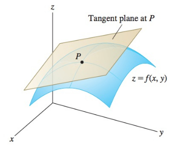
Fig. 50 Linear approximation of the a 3D surface with a tangent plane

Example

The second-order Taylor polynomial of a smooth function\(f:\mathbb R^N\to\mathbb R\)

Let \(\boldsymbol{x}-\boldsymbol{a}=\boldsymbol{v}\)

\[P_2(x) = f(\boldsymbol{a}) + \nabla f(\boldsymbol{a}) \boldsymbol{v} + \frac{1}{2} \boldsymbol{v}^T Hf(\boldsymbol{a}) \boldsymbol{v}\]

Example

The third-order Taylor polynomial of a smooth function\(f:\mathbb R^2\to\mathbb R\)

Let \(\boldsymbol{x}-\boldsymbol{a}=\boldsymbol{v}\)

\[\begin{split}\begin{align} P_3(\boldsymbol{x}) = f ( \boldsymbol{a} ) + {} &\frac{\partial f}{\partial x_1}( \boldsymbol{a} ) v_1 + \frac{\partial f}{\partial x_2}( \boldsymbol{a} ) v_2 + \frac{\partial^2 f}{\partial x_1^2}( \boldsymbol{a} ) \frac {v_1^2}{2!} + \frac{\partial^2 f}{\partial x_1 \partial x_2}( \boldsymbol{a} ) v_1 v_2 + \frac{\partial^2 f}{\partial x_2^2}( \boldsymbol{a} ) \frac{v_2^2}{2!} \\ & + \frac{\partial^3 f}{\partial x_1^3}( \boldsymbol{a} ) \frac{v_1^3}{3!} + \frac{\partial^3 f}{\partial x_1^2 \partial x_2}( \boldsymbol{a} ) \frac{v_1^2 v_2}{2!} + \frac{\partial^3 f}{\partial x_1 \partial x_2^2}( \boldsymbol{a} ) \frac{v_1 v_2^2}{2!} + \frac{\partial^3 f}{\partial x_2^3}( \boldsymbol{a} ) \frac{v_2^3}{3!} \end{align}\end{split}\]

Source: Wiki

Notes from the lecture

Hand written notes from the lecture

References and further reading

References

• [Simon and Blume, 1994]: Chapter 8