📖 Elements of linear algebra

Welcome back to face-to-face lecture! 😃
- Next test will be harder!
Online test: great results, congratulations! 🎉
- There were some issues with automatic grading such as misspelled contradiction
- errors corrected, grades updated 👍
Please check your grades and let us know if there are any issues

📖 Elements of linear algebra#

⏱ | words

Plan for the next couple lectures:

learn the concepts and the tools needed to work with multivariate optimization problems

put deeper meaning in matrix algebra by understanding the link between matrices and mappings

realize that matrices can be about anything

learn how to solve systems of linear equations along the way

Topics from linear algebra that we cover:

Vector space

Linear combination

Span

Linear independence

Basis and dimension

Matrices as linear transformations

Column spaces and null space

Rank of a matrix

Singular matrices

Euclidean space

Inner product and norm

Orthogonality

Change of basis

Eigenvectors and eigenvalues

Diagonalization of matrices

Diagonalization of symmetric matrices

Motivating example#

The most obvious application of linear algebra is solving systems of linear equations

Definition

A general system of linear equations can be written as

\[\begin{split} \begin{array}{c} a_{11} x_1 + a_{12} x_2 + \cdots + a_{1m} x_m = b_1 \\ a_{21} x_1 + a_{22} x_2 + \cdots + a_{2m} x_m = b_2 \\ \vdots \\ a_{n1} x_1 + a_{n2} x_2 + \cdots + a_{nm} x_m = b_n \end{array} \end{split}\]

More often we write the system in matrix form

\[\begin{split} \left( \begin{array}{cccc} a_{11} & a_{12} & \cdots & a_{1m} \\ a_{21} & a_{22} & \cdots & a_{2m} \\ \vdots & \vdots & & \vdots \\ a_{n1} & a_{n2} & \cdots & a_{nm} \end{array} \right) \left( \begin{array}{c} x_1 \\ x_2 \\ \vdots \\ x_m \end{array} \right) = \left( \begin{array}{c} b_1 \\ b_2 \\ \vdots \\ b_m \end{array} \right) % \end{split}\]

\[ % A x = b % \]

Let’s solve this system on a computer:

import numpy as np
from scipy.linalg import solve
A = [[0, 2, 4],
     [1, 4, 8],
     [0, 3, 7]]
b = (1, 2, 0)
A, b = np.asarray(A), np.asarray(b)
x=solve(A, b)
print(f'Solutions is x={x}')

Solutions is x=[-1.77635684e-15  3.50000000e+00 -1.50000000e+00]

This tells us that the solution is $x = (0 , 3.5, -1.5)$

That is,

\[\begin{split} % x = \left( \begin{array}{c} x_1 \\ x_2 \\ x_3 \end{array} \right) = \left( \begin{array}{r} 0 \\ 3.5 \\ -1.5 \end{array} \right) % \end{split}\]

The usual question: if computers can do it so easily — what do we need to study for?

But now let’s try this similar looking problem

Question: what changed?

import numpy as np
from scipy.linalg import solve
A = [[0, 2, 4],
     [1, 4, 8],
     [0, 3, 6]]
b = (1, 2, 0)
A, b = np.asarray(A), np.asarray(b)
x=solve(A, b)
print(f'Solutions is x={x}')

---------------------------------------------------------------------------
LinAlgError                               Traceback (most recent call last)
Cell In[2], line 8
      6 b = (1, 2, 0)
      7 A, b = np.asarray(A), np.asarray(b)
----> 8 x=solve(A, b)
      9 print(f'Solutions is x={x}')

File /opt/hostedtoolcache/Python/3.11.11/x64/lib/python3.11/site-packages/scipy/linalg/_basic.py:265, in solve(a, b, lower, overwrite_a, overwrite_b, check_finite, assume_a, transposed)
    262 gecon, getrf, getrs = get_lapack_funcs(('gecon', 'getrf', 'getrs'),
    263                                        (a1, b1))
    264 lu, ipvt, info = getrf(a1, overwrite_a=overwrite_a)
--> 265 _solve_check(n, info)
    266 x, info = getrs(lu, ipvt, b1,
    267                 trans=trans, overwrite_b=overwrite_b)
    268 _solve_check(n, info)

File /opt/hostedtoolcache/Python/3.11.11/x64/lib/python3.11/site-packages/scipy/linalg/_basic.py:42, in _solve_check(n, info, lamch, rcond)
     40     raise ValueError(f'LAPACK reported an illegal value in {-info}-th argument.')
     41 elif 0 < info:
---> 42     raise LinAlgError('Matrix is singular.')
     44 if lamch is None:
     45     return

LinAlgError: Matrix is singular.

This is the output that we get: LinAlgWarning: Ill-conditioned matrix

What does this mean?
How can we fix it?

We still need to understand the concepts after all!

Vector Space#

Definition

A field (of numbers) is a set $\mathbb{F}$ of numbers with the property that if $a,b \in \mathbb{F}$, then $a+b$, $a-b$, $ab$ and $a/b$ (provided that $b \ne 0$) are also in $\mathbb{F}$.

Example

$\mathbb{Q}$ and $\mathbb{R}$ are fields, but $\mathbb{N}$, $\mathbb{Z}$ is not (why?)

Definition

A vector space over a field $\mathbb{F}$ is a set $V$ of objects called vectors, together with two operations:

vector addition that takes two vectors $v,w \in V$ and produces a vector $v+w \in V$, and
scalar multiplication that takes a scalar $\alpha \in \mathbb{F}$ and a vector $v \in V$ and produces a vector $\alpha v \in V$,

which satisfy the following properties:

Commutativity of vector addition: $u+v = v+u$ all $u,v \in V$
Associativity of vector addition: $(u+v)+w = u+ (v+w)$ for all $u,v,w \in V$
Existance of identity element of vector addition (zero vector) ${\bf 0}$ such that $v + {\bf 0} = v$
Existance of additive inverse (negative vectors): for each $v \in V$ there exists a vector $-v \in V$ such that $v + (-v) = {\bf 0}$
Associativity of multiplication: $\alpha (\beta v) = (\alpha \beta) v$ for all $\alpha, \beta \in \mathbb{F}$ and $v \in V$
Identity element of scalar multiplication: $1v = v$ for all $v \in V$
Distributivity of scalar multiplication with respect to vector addition: $\alpha (v+w) = \alpha v + \alpha w$ for all $\alpha \in \mathbb{F}$ and $v, w \in V$
Distributivity of scalar multiplication with respect to field addition: $(\alpha + \beta) v = \alpha v + \beta v$ for all $\alpha, \beta \in \mathbb{F}$ and $v \in V$

may seem like a bunch of abstract nonsense, but it’s actually describes something intuitive
what we already know about operations with vectors in $\mathbb{R}^n$ put in formal definition

Example

\[\begin{split} % \left( \begin{array}{c} 1 \\ 2 \\ 3 \\ 4 \end{array} \right) + \left( \begin{array}{c} 2 \\ 4 \\ 6 \\ 8 \end{array} \right) = \left( \begin{array}{c} 3 \\ 6 \\ 9 \\ 12 \end{array} \right) % \end{split}\]

Example

\[\begin{split} % -1 \left( \begin{array}{c} 1 \\ 2 \\ 3 \\ 4 \end{array} \right) = \left( \begin{array}{c} -1 \\ -2 \\ -3 \\ -4 \end{array} \right) % \end{split}\]

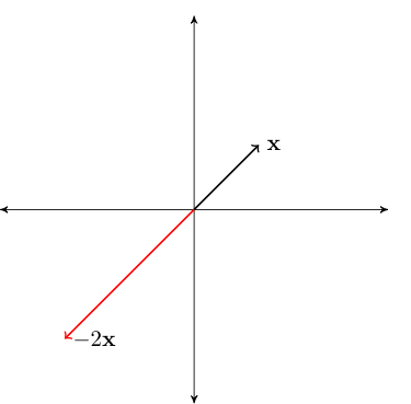
_images/vec_scalar.png — Fig. 33 Scalar multiplication by a negative number#

Example

$\mathbb{R}^n$ is a vector space

Example

The space of polynomials up to degree $m$. Typical element is

\[ p(x) = a_m x^m + a_{m-1} x^{m-1} + \dots + a_1 x + a_0 \]

You can check that with neutral elements equal to $p_0(x)=0$ all properties of vector space are satisfied

Linear combinations#

Definition

A linear combination of vectors $x_1,\ldots, x_m$ in $\mathbb{R}^n$ is a vector

\[ % y = \sum_{j=1}^m \alpha_j x_j = \alpha_1 x_1 + \cdots + \alpha_m x_m % \]

where $\alpha_1,\ldots, \alpha_m$ are scalars

Example

\[\begin{split} % 0.5 \left( \begin{array}{r} 6 \\ 2 \\ 8 \end{array} \right) + 3 \left( \begin{array}{r} 0 \\ 1 \\ -1 \end{array} \right) = \left( \begin{array}{r} 3 \\ 4 \\ 1 \end{array} \right) % \end{split}\]

\[\begin{split} \left( \begin{array}{r} 3 \\ 4 \\ 1 \end{array} \right) \; \text{is a linear combination of} \; \left( \begin{array}{r} 6 \\ 2 \\ 8 \end{array} \right) \;\text{and}\; \left( \begin{array}{r} 0 \\ 1 \\ -1 \end{array} \right) \end{split}\]

Span#

Let $X \subset \mathbb{R}^n$ be any nonempty set (of points in $\mathbb{R}^n$, i.e. vectors)

Definition

A set of all possible linear combinations of elements of $X$ is called the span of $X$, denoted by $\mathrm{span}(X)$

For finite $X = \{x_1,\ldots, x_m\}$ the span can be expressed as

\[ \mathrm{span}(X)= \left\{ y = \sum_{j=1}^m \alpha_j x_j \text{ for all } (\alpha_1,\ldots, \alpha_m) \in \mathbb{R}^m \right\} \]

Example

Let’s start with the span of a singleton

Let $X = \{ (1,1) \} \subset \mathbb{R}^2$

The span of $X$ is all vectors of the form

\[\begin{split} % \left( \begin{array}{c} \alpha \\ \alpha \end{array} \right) \quad \text{ with } \quad \alpha \in \mathbb{R} % \end{split}\]

Constitutes a line in the plane that passes through

the vector $(1,1)$ (set $\alpha = 1$)
the origin $(0,0)$ (set $\alpha = 0$)

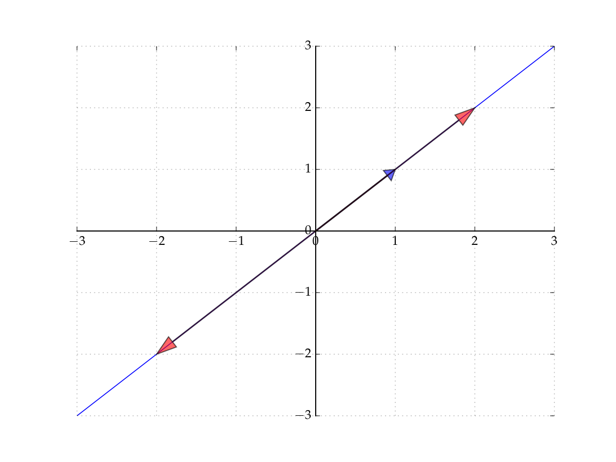
_images/span_of_one_vec.png — Fig. 34 The span of $(1,1)$ in $\mathbb{R}^2$#

Example

Let $x_1 = (3, 4, 2)$ and let $x_2 = (3, -4, 0.4)$

By definition, the span is all vectors of the form

\[\begin{split} % y = \alpha \left( \begin{array}{c} 3 \\ 4 \\ 2 \end{array} \right) + \beta \left( \begin{array}{c} 3 \\ -4 \\ 0.4 \end{array} \right) \quad \text{where} \quad \alpha, \beta \in \mathbb{R} % \end{split}\]

It turns out to be a plane that passes through

the vector $x_1$
the vector $x_2$
the origin ${\bf 0}$

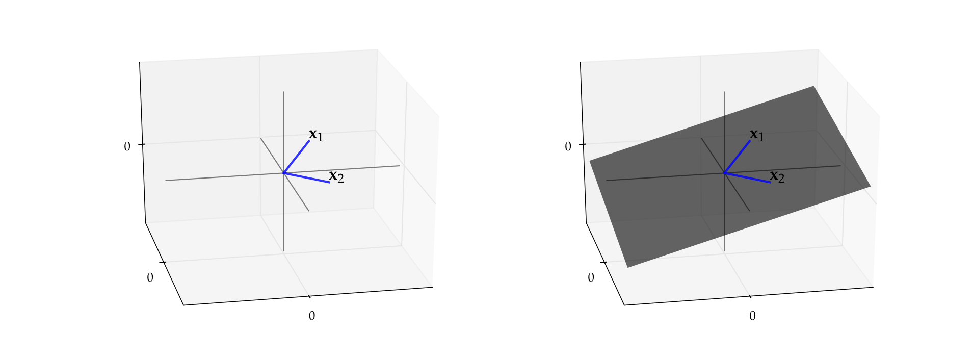
_images/span_plane.png — Fig. 35 Span of $\{x_1, x_2\}$ in $\mathbb{R}^3$ is a plane#

Definition

Consider the vectors $\{e_1, \ldots, e_n\} \subset \mathbb{R}^n$, where

\[\begin{split} % e_1 = \left( \begin{array}{c} 1 \\ 0 \\ \vdots \\ 0 \end{array} \right), \quad e_2 = \left( \begin{array}{c} 0 \\ 1 \\ \vdots \\ 0 \end{array} \right), \; \cdots, \; e_n = \left( \begin{array}{c} 0 \\ 0 \\ \vdots \\ 1 \end{array} \right) % \end{split}\]

That is, $e_n$ has all zeros except for a $1$ as the $n$-th element

Vectors $e_1, \ldots, e_n$ are called the canonical basis vectors of $\mathbb{R}^n$

_images/vec_canon.png — Fig. 36 Canonical basis vectors in $\mathbb{R}^2$#

Fact

The span of $\{e_1, \ldots, e_n\}$ is equal to all of $\mathbb{R}^n$

Proof

Proof for $n=2$:

Pick any $y \in \mathbb{R}^2$

We have

\[\begin{split} % y = \left( \begin{array}{c} y_1 \\ y_2 \end{array} \right) = \left( \begin{array}{c} y_1 \\ 0 \end{array} \right) + \left( \begin{array}{c} 0 \\ y_1 \end{array} \right) \\ = y_1 \left( \begin{array}{c} 1 \\ 0 \end{array} \right) + y_2 \left( \begin{array}{c} 0 \\ 1 \end{array} \right) = y_1 e_1 + y_2 e_2 % \end{split}\]

Thus, $y \in \mathrm{span} \{e_1, e_2\}$

Since $y$ arbitrary, we have shown that $\mathrm{span} \{e_1, e_2\} = \mathbb{R}^2$

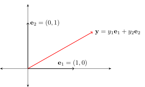
_images/vec_canon_x.png — Fig. 37 Canonical basis vectors in $\mathbb{R}^2$#

Linear subspace#

Definition

A nonempty $S \subset \mathbb{R}^n$ called a linear subspace of $\mathbb{R}^n$ if

\[ % x, y \in S \; \text{ and } \;\alpha, \beta \in \mathbb{R} \quad \implies \quad \alpha x + \beta y \in S % \]

In other words, $S \subset \mathbb{R}^n$ is “closed” under vector addition and scalar multiplication

Note: Sometimes we just say subspace and drop “linear”

Example

$\mathbb{R}^n$ itself is a linear subspace of $\mathbb{R}^n$

Linear independence#

Definition

A nonempty collection of vectors $X = \{x_1,\ldots, x_m\} \subset \mathbb{R}^n$ is called linearly independent if

\[ % \sum_{j=1}^m \alpha_j x_j = {\bf 0} \; \implies \; \alpha_1 = \cdots = \alpha_m = 0 % \]

Equivalently

\[\begin{split} a^T x = {\bf 0} \; \implies \; \left( \begin{array}{c} a_1 \\ \vdots \\ a_m \end{array} \right) =\left( \begin{array}{c} 0 \\ \vdots \\ 0 \end{array} \right) \end{split}\]

the notation $\square^T$ is transposition operation which flips the vector from column-vector to row-vector to allow for standard matrix application to apply
linear independence of a set of vectors determines how large a space they span
loosely speaking, linearly independent sets span larger spaces than linearly dependent

Example

Let $x = (1, 2)$ and $y = (-5, 3)$

The set $X = \{x, y\}$ is linearly independent in $\mathbb{R}^2$

Indeed, suppose $\alpha_1$ and $\alpha_2$ are scalars with

\[\begin{split} % \alpha_1 \left( \begin{array}{c} 1 \\ 2 \end{array} \right) + \alpha_2 \left( \begin{array}{c} -5 \\ 3 \end{array} \right) = {\bf 0} \end{split}\]

Equivalently, $$ \alpha_1 = 5 \alpha_2 \\ 2 \alpha_1 = -3 \alpha_2 $$

Then $2(5\alpha_2) = 10 \alpha_2 = -3 \alpha_2$, implying $\alpha_2 = 0$ and hence $\alpha_1 = 0$

Fact

The set of canonical basis vectors $\{e_1, \ldots, e_n\}$ is linearly independent in $\mathbb{R}^n$

Proof

Let $\alpha_1, \ldots, \alpha_n$ be coefficients such that $\sum_{k=1}^n \alpha_j e_j = {\bf 0}$

Then

\[\begin{split} \left( \begin{array}{c} 0 \\ 0 \\ \vdots \\ 0 \end{array} \right) = \big( \alpha_1, \alpha_2, \dots, \alpha_n \big) \left( \begin{array}{cccc} 1,&0,&\dots&0\\ 0,&1,&\dots&0\\ \vdots&\vdots&\ddots&\vdots\\ 0,&0,&\dots&1 \end{array} \right) = \left( \begin{array}{c} \alpha_1 \\ \alpha_2 \\ \vdots \\ \alpha_n \end{array} \right) % \end{split}\]

In particular, $\alpha_j = $ for all $k$

Hence $\{e_1, \ldots, e_n\}$ linearly independent

$\blacksquare$

Fact

Take $X = \{x_1,\ldots, x_m\} \subset \mathbb{R}^n$. For $m > 1$ all of following statements are equivalent

$X$ is linearly independent

$\quad\quad\Updownarrow$

No $x_j \in X$ can be written as linear combination of the others

$\quad\quad\Updownarrow$

$X_0 \subset X \implies \mathrm{span}(X_0) \subset \mathrm{span}(X)$

Example

As another visual example of linear independence, consider the pair

\[\begin{split} % x_1 = \begin{pmatrix} 3 \\ 4 \\ 2 \end{pmatrix} \quad \text{and} \quad x_2 = \begin{pmatrix} 3 \\ -4 \\ 1 \end{pmatrix} % \end{split}\]

The span of this pair is a plane in $\mathbb{R}^3$

But if we drop either one the span reduces to a line

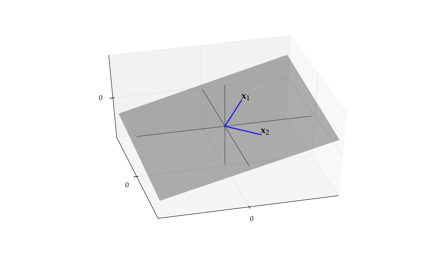
_images/nonredundant1.png — Fig. 38 The span of $\{x_1, x_2\}$ is a plane#

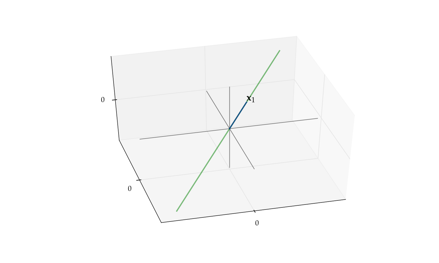
_images/nonredundant2.png — Fig. 39 The span of $\{x_1\}$ alone is a line#

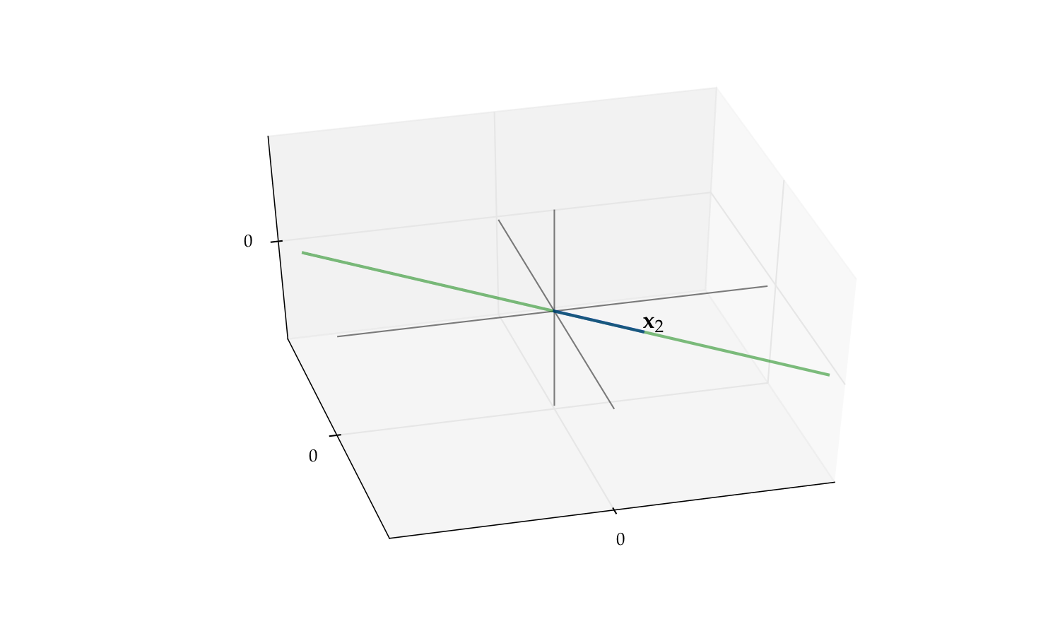
_images/nonredundant3.png — Fig. 40 The span of $\{x_2\}$ alone is a line#

Fact

If set $X$ is linearly independent, then $X$ does not contain zero vector ${\bf 0}$

Proof

Exercise

Fact

If $X$ is linearly independent, then every subset of $X$ is linearly independent

Proof

Sketch of proof: Suppose for example that $\{x_1,\ldots, x_{m-1}\} \subset X$ is linearly dependent

Then $\exists \; \alpha_1, \ldots, \alpha_{m-1}$ not all zero with $\sum_{k=1}^{m-1} \alpha_j x_j = 0$

Setting $\alpha_m =0$ we can write this as $\sum_{j=1}^m \alpha_j x_j = {\bf 0}$, where not all scalars zero so contradicts linear independence of $X$

Fact

If $X= \{x_1,\ldots, x_m\} \subset \mathbb{R}^n$ is linearly independent and $z$ is an $n$-vector not in $\mathrm{span}(X)$ then $X \cup \{ z \}$ is linearly independent

Proof

Suppose to the contrary that $X \cup \{ z \}$ is linearly dependent:

\[ % \exists \; \alpha_1, \ldots, \alpha_m, \beta \text{ not all zero with } \sum_{j=1}^m \alpha_j x_j + \beta z = {\bf 0} % \]

If $\beta$ was zero, it would imply that some of the $\alpha_j$ is not zero, contradicting linear independence of $X$.

Thus, $\beta \ne0$. Then by we have

\[ % z = \sum_{j=1}^m \frac{-\alpha_j}{\beta} x_j % \]

Hence $z \in \mathrm{span}(X)$ — contradiction

Fact

If $X = \{x_1,\ldots, x_m\} \subset \mathbb{R}^n$ is linearly independent and $y \in \mathbb{R}^n$, then there is at most one set of scalars $\alpha_1,\ldots,\alpha_m$ such that $y = \sum_{j=1}^m \alpha_j x_j$

Proof

Suppose there are two such sets of scalars

That is,

\[ % \exists \; \alpha_1, \ldots, \alpha_m \text{ and } \beta_1, \ldots, \beta_m \; \text{ such that } \; y = \sum_{j=1}^m \alpha_j x_j = \sum_{j=1}^m \beta_j x_j % \]

\[ % \implies \sum_{j=1}^m (\alpha_j - \beta_j) x_j = {\bf 0} % \]

\[ % \implies \alpha_j = \beta_j \; \text{for all} \; j % \]

due to linear independence of $X$

Here’s one of the most fundamental results in linear algebra

It connects:

linear subspace
span
linear independence

Exchange Lemma

Let $X$ be a linear subspace of $\mathbb{R}^n$, and be spanned by $K$ vectors
(that is $\exists K$ vectors whose span is equal to the initial subspace).
Then any linearly independent subset of $X$ has at most $K$ vectors.

Example

If $X = \{x_1, x_2, x_3\} \subset \mathbb{R}^2$, then $X$ is linearly dependent

because $\mathbb{R}^2$ is spanned by the two vectors $e_1, e_2$

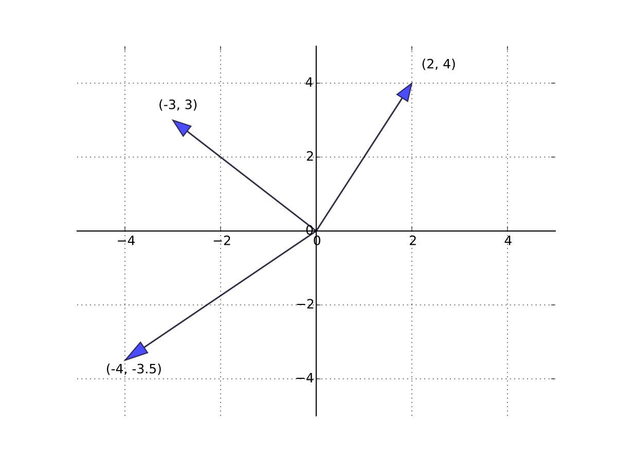
_images/vecs.png — Fig. 41 Must be linearly dependent#

Fact

Let $X = \{ x_1, \ldots, x_n \}$ be any $n$ vectors in $\mathbb{R}^n$

$\mathrm{span}(X) = \mathbb{R}^n$ if and only if $X$ is linearly independent

Example

The vectors $x = (1, 2)$ and $y = (-5, 3)$ span $\mathbb{R}^2$

Proof

Let prove that

$X= \{ x_1, \ldots, x_n \}$ linearly independent $\implies$ $\mathrm{span}(X) = \mathbb{R}^n$

Seeking a contradiction, suppose that

$X $ is linearly independent
and yet $\exists \, z \in \mathbb{R}^n$ with $z \notin \mathrm{span}(X)$

But then $X \cup \{z\} \subset \mathbb{R}^n$ is linearly independent (why?)

This set has $n+1$ elements

And yet $\mathbb{R}^n$ is spanned by the $n$ canonical basis vectors

Contradiction (of what?)

Next let’s show the converse

$\mathrm{span}(X) = \mathbb{R}^n$ $\implies$ $X= \{ x_1, \ldots, x_n \}$ linearly independent

Seeking a contradiction, suppose that

$\mathrm{span}(X) = \mathbb{R}^n$
and yet $X$ is linearly dependent

Since $X$ not independent, $\exists X_0 \subsetneq X$ with $\mathrm{span}(X_0) = \mathrm{span}(X)$

But by 1 this implies that $\mathbb{R}^n$ is spanned by $K < n$ vectors

But then the $n$ canonical basis vectors must be linearly dependent

Contradiction

Bases and dimension#

Definition

Let $S$ be a linear subspace of $\mathbb{R}^n$

A set of vectors $B = \{b_1, \ldots, b_m\} \subset S$ is called a basis of $S$ if

$B$ is linearly independent
$\mathrm{span}(B) = S$

Example

Canonical basis vectors form a basis of $\mathbb{R}^n$

Example

Recall the plane

\[ % P = \{ (x_1, x_2, 0) \in \mathbb{R}^3 \colon x_1, x_2 \in \mathbb{R \}} % \]

We can show that $\mathrm{span}\{e_1, e_2\} = P$ for

\[\begin{split} % e_1 = \left( \begin{array}{c} 1 \\ 0 \\ 0 \end{array} \right), \quad e_2 = \left( \begin{array}{c} 0 \\ 1 \\ 0 \end{array} \right) % \end{split}\]

Moreover, $\{e_1, e_2\}$ is linearly independent (why?)

Hence $\{e_1, e_2\}$ is a basis for $P$

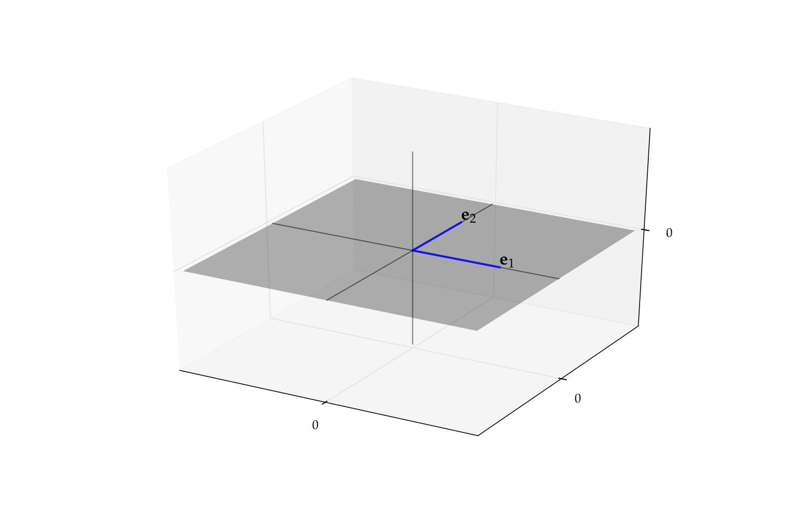
_images/flat_plane_e_vecs.png — Fig. 42 The pair $\{e_1, e_2\}$ form a basis for $P$#

What are the implications of $B$ being a basis of $S$?

every element of $S$ can be represented uniquely from the smaller set $B$

In more detail:

$B$ spans $S$ and, by linear independence, every element is needed to span $S$ — a “minimal” spanning set
Since $B$ spans $S$, every $y$ in $S$ can be represented as a linear combination of the basis vectors
By independence, this representation is unique

Fact

If $B \subset \mathbb{R}^n$ is linearly independent, then $B$ is a basis of $\mathrm{span}(B)$

Proof

Follows from the definitions

Fact: Fundamental Properties of Bases

If $S$ is a linear subspace of $\mathbb{R}^n$ distinct from $\{{\bf 0}\}$, then

$S$ has at least one basis, and
every basis of $S$ has the same number of elements

Proof

Proof of part 2: Let $B_i$ be a basis of $S$ with $K_i$ elements, $i=1, 2$

By definition, $B_2$ is a linearly independent subset of $S$

Moreover, $S$ is spanned by the set $B_1$, which has $K_1$ elements

Hence $K_2 \leq K_1$

Reversing the roles of $B_1$ and $B_2$ gives $K_1 \leq K_2$

Definition

Let $S$ be a linear subspace of $\mathbb{R}^n$

We now know that every basis of $S$ has the same number of elements

This common number is called the dimension of $S$

Example

$\mathbb{R}^n$ is $n$ dimensional because the $n$ canonical basis vectors form a basis

Example

$P = \{ (x_1, x_2, 0) \in \mathbb{R}^3 \colon x_1, x_2 \in \mathbb{R \}}$ is two dimensional because the first two canonical basis vectors of $\mathbb{R}^3$ form a basis

Linear Functions#

Very useful:

We’ll see that linear functions are in one-to-one correspondence with matrices
Nonlinear functions are closely connected to linear functions through Taylor approximation

Definition

A function $T \colon \mathbb{R}^m \to \mathbb{R}^n$ is called linear if

\[ % T(\alpha x + \beta y) = \alpha Tx + \beta Ty \qquad \forall \, x, y \in \mathbb{R}^m, \; \forall \, \alpha, \beta \in \mathbb{R} % \]

Linear functions are like matrix multiplication:

Linear functions are often written with upper case letters
Typically omit parenthesis around arguments when convenient
Bear in mind that $\mathbb{R}^n$ is a vector space

Example

$T \colon \mathbb{R} \to \mathbb{R}$ defined by $Tx = 2x$ is linear

Proof

Take any $\alpha, \beta, x, y$ in $\mathbb{R}$ and observe that

\[ % T(\alpha x + \beta y) = 2(\alpha x + \beta y) = \alpha 2 x + \beta 2 y = \alpha Tx + \beta Ty % \]

Example

The function $f \colon \mathbb{R} \to \mathbb{R}$ defined by $f(x) = x^2$ is nonlinear

Proof

It’s sufficient to find one counterexample. Set $\alpha = \beta = x = y = 1$

Then

$f(\alpha x + \beta y) = f(2) = 4$
But $\alpha f(x) + \beta f(y) = 1 + 1 = 2$

Example

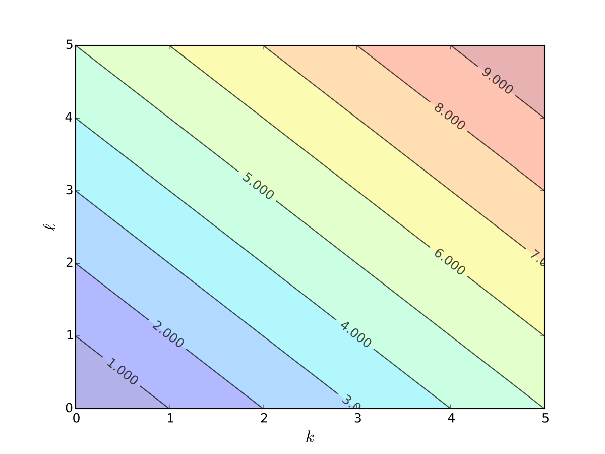
Given constants $c_1$ and $c_2$ in $\mathbb{R}$, the function $T \colon \mathbb{R}^2 \to \mathbb{R}$ defined by

\[ % T x = T (x_1, x_2) = c_1 x_1 + c_2 x_2 % \]

is linear

Proof

If we take any $\alpha, \beta$ in $\mathbb{R}$ and $x, y$ in $\mathbb{R}^2$, then

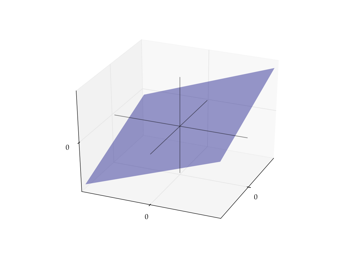
\[\begin{split} % T(\alpha x + \beta y) = c_1 [\alpha x_1 + \beta y_1] + c_2 [\alpha x_2 + \beta y_2] \\ = \alpha [c_1 x_1 + c_2 x_2] + \beta [c_1 y_1 + c_2 y_2] \\ = \alpha T x + \beta T y % \end{split}\]

_images/linfunc.png — Fig. 43 The graph of $T x = c_1 x_1 + c_2 x_2$ is a plane through the origin#

Thinking of linear functions as those whose graph is a straight line is not correct!

Example

Function $f \colon \mathbb{R} \to \mathbb{R}$ defined by $f(x) = 1 + 2x$ is nonlinear

Proof

Take $\alpha = \beta = x = y = 1$

Then

$f(\alpha x + \beta y) = f(2) = 5$
But $\alpha f(x) + \beta f(y) = 3 + 3 = 6$

This kind of function is called an affine function

Fact

If $T \colon \mathbb{R}^m \to \mathbb{R}^n$ is a linear mapping and $x_1,\ldots, x_J$ are vectors in $\mathbb{R}^m$, then for any linear combination we have

\[ T \left[ \alpha_1 x_1 + \cdots + \alpha_J x_J \right] = \alpha_1 T x_1 + \cdots + \alpha_J T x_J \]

generalization of the definition of linear functions

Proof

Can be proved by a repeated application of the definition of linearity.

Proof for $J=3$: Applying the definition twice,

\[\begin{split} % T \left[ \alpha_1 x_1 + \alpha_2 x_2 + \alpha_3 x_3 \right] = T\left[ (\alpha_1 x_1 + \alpha_2 x_2) + \alpha_3 x_3 \right] \\ = T\left[ \alpha_1 x_1 + \alpha_2 x_2 \right] + \alpha_3 T x_3 \\ = \alpha_1 T x_1 + \alpha_2 T x_2 + \alpha_3 T x_3 % \end{split}\]

The following very important result will be very useful in a moment:

Fact

If $T \colon \mathbb{R}^m \to \mathbb{R}^n$ is a linear mapping, then

\[ % \mathrm{rng}(T) = \mathrm{span}(V) \quad \text{where} \quad V = \{Te_1, \ldots, Te_m\} % \]

Here $e_j$ is the $j$-th canonical basis vector in $\mathbb{R}^m$

In other words, all the information about the linear mapping is contained in the image of the canonical basis vectors!

Proof

Any $x \in \mathbb{R}^m$ can be expressed as $\sum_{j=1}^m \alpha_j e_j$

Hence $\mathrm{rng}(T)$ is the set of all points of the form

\[ % Tx = T \left[ \sum_{j=1}^m \alpha_j e_j \right] = \sum_{j=1}^m \alpha_j T e_j % \]

as we vary $\alpha_1, \ldots, \alpha_m$ over all combinations.

This coincides with the definition of $\mathrm{span}(V)$!

Example

Let $T \colon \mathbb{R}^2 \to \mathbb{R}^2$ be defined by

\[\begin{split} % Tx = T(x_1, x_2) = x_1 \begin{pmatrix} 1 \\ 2 \end{pmatrix} + x_2 \begin{pmatrix} 0 \\ -2 \end{pmatrix} % \end{split}\]

Then

\[\begin{split} % Te_1 = \begin{pmatrix} 1 \\ 2 \end{pmatrix} \quad \text{and} \quad Te_2 = \begin{pmatrix} 0 \\ -2 \end{pmatrix} % \end{split}\]

We can show that $V = \{Te_1, Te_2\}$ is linearly independent similarly to above (exercise)

We conclude that the range of $T$ is all of $\mathbb{R}^2$ (why?)

Definition

The null space or kernel of linear mapping $T \colon \mathbb{R}^m \to \mathbb{R}^n$ is

\[ % \mathrm{kernel}(T) = \{ x \in \mathbb{R}^m \colon Tx = {\bf 0}\} % \]

Linearity and Bijections#

Recall that an arbitrary function can be

one-to-one (injections)
onto (surjections)
both (bijections)
neither

It turnes out that for linear functions from $\mathbb{R}^n$ to $\mathbb{R}^n$, the first three are all equivalent!

In particular, $$ \text{onto } \iff \text{ one-to-one } \iff \text{ bijection} $$

Fact

If $T$ is a linear function from $\mathbb{R}^n$ to $\mathbb{R}^n$ then all of the following are equivalent:

$T$ is a bijection

$\quad\quad\Updownarrow$

$T$ is onto/surjective

$\quad\quad\Updownarrow$

$T$ is one-to-one/injective

$\quad\quad\Updownarrow$

$\mathrm{kernel}(T) = \{ 0 \}$

$\quad\quad\Updownarrow$

The set of vectors $V = \{Te_1, \ldots, Te_n\}$ is linearly independent

Definition

If any one of the above equivalent conditions is true, then $T$ is called nonsingular

Proof

Proof that $T$ onto $\iff$ $V = \{Te_1, \ldots, Te_n\}$ is linearly independent

Recall that for any linear mapping $T$ we have $\mathrm{rng}(T) = \mathrm{span}(V)$

Using this fact and the definitions,

\[\begin{split} % T \text{ is onto/surjective } \iff \mathrm{rng}(T) = \mathbb{R}^n \\ \iff \mathrm{span}(V) = \mathbb{R}^n \\ \iff V \text{ is linearly indepenent} % \end{split}\]

(We saw that $n$ vectors span $\mathbb{R}^n$ iff linearly indepenent)

Exercise: rest of proof

Fact

If $T \colon \mathbb{R}^n \to \mathbb{R}^n$ is nonsingular then so is $T^{-1}$.

Proof

Exercise: prove this statement

Mappings Across Different Dimensions#

Remember that the above results apply to mappings from $\mathbb{R}^n$ to $\mathbb{R}^n$!

Things change when we look at linear mappings across dimensions. The general rules for linear mappings are:

Mappings from lower to higher dimensions cannot be onto
Mappings from higher to lower dimensions cannot be one-to-one
In either case they cannot be bijections

Fact

For a linear mapping $T$ from $\mathbb{R}^m \to \mathbb{R}^n$, the following statements are true:

If $m < n$ then $T$ is not onto
If $m > n$ then $T$ is not one-to-one

Proof

Proof of part 1: Let $m < n$ and let $T \colon \mathbb{R}^m \to \mathbb{R}^n$ be linear

Letting $V = \{Te_1, \ldots, Te_m\}$, we have

\[ \dim(\mathrm{rng}(T)) = \dim(\mathrm{span}(V)) \leq m < n \]

\[ % \implies \mathrm{rng}(T) \ne \mathbb{R}^n % \]

Hence $T$ is not onto

Proof of part 2:

Suppose to the contrary that $m>n$ but $T$ is one-to-one

Let $\alpha_1, \ldots, \alpha_m$ be a collection of vectors such that

\[ \alpha_1 T e_1 + \cdots + \alpha_m T e_m = 0 \]

\[ \implies T (\alpha_1 e_1 + \cdots + \alpha_m e_m) = 0 \qquad (\text{by linearity}) \]

\[ \implies \alpha_1 e_1 + \cdots + \alpha_m e_m = 0 \qquad (\text{since $\ker(T) = \{0\}$}) \]

\[ % \implies \alpha_1 = \cdots = \alpha_m = 0 \qquad (\text{by independence of $\{e_1, \ldots e_m\}$)} % \]

We have shown that $\{Te_1, \ldots, Te_m\}$ is linearly independent

But then $\mathbb{R}^n$ contains a linearly independent set with $m > n$ vectors — contradiction

Example

Cost function $c(k, \ell) = rk + w\ell$ cannot be one-to-one

Linear Functions are Matrix Multiplication#

First, any $n \times m$ matrix $A$ can be thought of as a function

\[ \mathbb{R}^m \ni x \mapsto A x \in \mathbb{R}^n \]

in $A x$ the $x$ is understood to be a column vector

Fact

Every function of the form

\[ T \colon \mathbb{R}^m \to \mathbb{R}^n, \qquad Tx = A x \]

where $A$ is an $n \times m$ matrix, is linear

Proof

Pick any $x$, $y$ in $\mathbb{R}^m$, and any scalars $\alpha$ and $\beta$

The rules of matrix arithmetic tell us that

\[ T(\alpha x + \beta y) = A (\alpha x + \beta y) = \alpha A x + \beta A y =: \alpha Tx + \beta Ty \]

$\blacksquare$

So matrices make linear functions

How about examples of linear functions that don’t involve matrices?

There are none!

Fact

Every linear function $T \colon \mathbb{R}^m \to \mathbb{R}^n$ can be expressed as matrix multiplication

\[ T \text{ is linear } \; \iff \; \exists \; n \times m \text{ matrix } A \text{ such that } Tx = Ax, \;\forall \, x \in \mathbb{R}^m \; \text{(column vector)} \]

Proof

In previous fact above we showed the $\Longleftarrow$ part
Let’s show the $\implies$ part

Let $T \colon \mathbb{R}^m \to \mathbb{R}^n$ be linear

We aim to construct an $n \times m$ matrix $A$ such that

\[ Tx = A x, \qquad \forall \, x \in \mathbb{R}^m \]

As usual, let $e_j$ be the $j$-th canonical basis vector in $\mathbb{R}^m$

Define a matrix $A$ by $\mathrm{col}_j(A) = Te_j$, that is form matrix $A$ from $m$ column vectors $Te_j$

Pick any $x = (x_1, \ldots, x_m) \in \mathbb{R}^m$

By linearity we have

\[ % Tx = T \left[\sum_{j=1}^m x_j e_j \right] = \sum_{j=1}^m x_j T e_j = \sum_{j=1}^m x_j \mathrm{col}_j(A) = A x % \]

$\blacksquare$

Matrix Product as Composition#

Fact

Let matrices $A$ be $n \times m$ and $B$ be $m \times k$.

Consider

$T \colon \mathbb{R}^m \to \mathbb{R}^n$ be the linear mapping $Tx = Ax$
$U \colon \mathbb{R}^k \to \mathbb{R}^m$ be the linear mapping $Ux = Bx$

The matrix product $A B$ corresponds exactly to the composition of mappings $T$ and $U$:

\[ \mathbb{R}^k \ni x \mapsto (T \circ U) (x) = A B x \in \mathbb{R}^n \]

Proof

Substitute the definitions of the two mappings

\[ (T \circ U) (x) = T( Ux) = T( B x) = A B x \]

Column Space#

Definition

Let $A$ be an $n \times m$ matrix. The column space of $A$ is defined as the span of its columns

\[ \mathrm{span}(A) = \mathrm{span} \Big\{ \mathrm{col}_1 (A), \ldots, \mathrm{col}_m(A) \Big\} = \left\{y\in\mathbb{R}^n:\; y=\sum_{j=1}^m x_j \mathrm{col}_j(A)\; \forall x \in \mathbb{R}^m\right\} \]

Equivalently, $$ \mathrm{span}(A) = \{ Ax \colon\; \forall x \in \mathbb{R}^m \} $$

This is exactly the range of the associated linear mapping

$T \colon \mathbb{R}^m \to \mathbb{R}^n$ defined by $T x = A x$

Example

If

\[\begin{split} % A = \begin{pmatrix} 1 & -5 \\ 2 & 3 \end{pmatrix} % \end{split}\]

then the span is all linear combinations

\[\begin{split} % x_1 \left( \begin{array}{c} 1 \\ 2 \end{array} \right) + x_2 \left( \begin{array}{c} -5 \\ 3 \end{array} \right) \quad \text{where} \quad (x_1, x_2) \in \mathbb{R}^2 % \end{split}\]

These columns are linearly independent (shown earlier)

Hence the column space is all of $\mathbb{R}^2$ (why?)

Exercise: Show that the column space of any $n \times m$ matrix is a linear subspace of $\mathbb{R}^n$

Rank#

Equivalent questions

How large is the range of the linear mapping $T x = A x$?
How large is the column space of $A$?

The obvious measure of size for a linear subspace is its dimension

Definition

The dimension of $\mathrm{span}(A)$ is known as the rank of $A$

\[ % \mathrm{rank}(A) = \mathrm{dim}(\mathrm{span}(A)) % \]

Because $\mathrm{span}(A)$ is the span of $K$ vectors, we have

\[ % \mathrm{rank}(A) = \mathrm{dim}(\mathrm{span}(A)) \leq K % \]

Definition

$A$ is said to have full column rank if

\[ % \mathrm{rank}(A) = \text{ number of columns of } A % \]

Fact

For any matrix $A$, the following statements are equivalent:

$A$ is of full column rank

$\quad\quad\Updownarrow$

The columns of $A$ are linearly independent

$\quad\quad\Updownarrow$

If $A x = 0$, then $x = 0$

Exercise: Check this, recalling that

\[ % \dim(\mathrm{span}\{a_1, \ldots, a_m\}) = K \, \iff \, \{a_1, \ldots, a_m\} \text{ linearly indepenent} % \]

import numpy as np
A = [[2.0, 1.0],
     [6.5, 3.0]]
print(f'Rank = {np.linalg.matrix_rank(A)}')
A = [[2.0, 1.0],
     [6.0, 3.0]]
print(f'Rank = {np.linalg.matrix_rank(A)}')

Systems of Linear Equations#

Back to the motivating example!

Let’s look at solving linear equations such as $A x = b$ where $A$ is a square matrix $n \times n$

Take $n \times n$ matrix $A$ and $n \times 1$ vector $b$ as given
Search for an $n \times 1$ solution $x$

But does such a solution exist? If so is it unique?

The best way to think about this is to consider the corresponding linear mapping

\[ % T \colon \mathbb{R}^n \ni x \mapsto Tx = A x \in \mathbb{R}^n % \]

Note the equivalence:

$A x = b$ has a unique solution $x$ for any given $b$

$\quad\quad\Updownarrow$

$T x = b$ has a unique solution $x$ for any given $b$

$\quad\quad\Updownarrow$

$T$ is a bijection

We already have conditions for linear mappings to be bijections

Just need to translate these into the matrix setting

Recall that linear mapping $T$ is called nonsingular if $T$ is a linear bijection

Definition

We say that $A$ is nonsingular if $T: x \to Ax$ is nonsingular

Equivalent: $x \mapsto A x$ is a bijection from $\mathbb{R}^n$ to $\mathbb{R}^n$

We now list equivalent conditions for nonsingularity

Fact

Let $A$ be an $n \times n$ matrix
All of the following conditions are equivalent

$A$ is nonsingular

$\quad\quad\Updownarrow$

The columns of $A$ are linearly independent

$\quad\quad\Updownarrow$

$\mathrm{rank}(A) = n$

$\quad\quad\Updownarrow$

$\mathrm{span}(A) = \mathbb{R}^n$

$\quad\quad\Updownarrow$

If $A x = A y$, then $x = y$

$\quad\quad\Updownarrow$

If $A x = 0$, then $x = 0$

$\quad\quad\Updownarrow$

For each $b \in \mathbb{R}^n$, the equation $A x = b$ has a solution

$\quad\quad\Updownarrow$

For each $b \in \mathbb{R}^n$, the equation $A x = b$ has a unique solution

All equivalent ways of saying that $Tx = A x$ is a bijection!

Example

For condition 5 the equivalence is:
$A x = A y$, then $x = y$ $\iff$ $T x = T y$, then $x = y$ $\iff$ $T$ is one-to-one $\iff$ Since $T$ is a linear mapping from $\mathbb{R}^n$ to $\mathbb{R}^n$, $T$ is a bijection

Example

For condition 6 the equivalence is:
if $A x = 0$, then $x = 0$ $\iff$ $\{x: Ax = 0\} = \{0\}$ $\iff$ $\{x: Tx = 0\} = \{0\}$ $\iff$ $\ker{T}=\{0\}$ $\iff$ Since $T$ is a linear mapping from $\mathbb{R}^n$ to $\mathbb{R}^n$, $T$ is a bijection

Example

For condition 7 the equivalence is:
for each $b\in\mathbb{R}^n$, the equation $Ax = b$ has a solution $\iff$ every $b\in\mathbb{R}^n$ has an $x$ such that $Ax = b$ $\iff$ every $b\in\mathbb{R}^n$ has an $x$ such that $Tx = b$ $\iff$ $T$ is onto/surjection $\iff$ Since $T$ is a linear mapping from $\mathbb{R}^n$ to $\mathbb{R}^n$, $T$ is a bijection

Example

Now consider condition 2: \

The columns of $A$ are linearly independent.

Let $e_j$ be the $j$-th canonical basis vector in $\mathbb{R}^n$.

Observe that $Ae_j = \mathrm{col}_j(A)$ $\implies$ $Te_j = \mathrm{col}_j(A)$ $\implies$ $V = \{T e_1, \ldots, Te_n\} =$ columns of $A$, and $V$ is linearly independent if and only if $T$ is a bijection

Example

Consider a one good linear market system

\[\begin{split} % q = a - b p \qquad (\text{demand}) \\ q = c + d p \qquad (\text{supply}) % \end{split}\]

Treating $q$ and $p$ as the unknowns, let’s write in matrix form as

\[\begin{split} % \begin{pmatrix} 1 & b \\ 1 & -d \end{pmatrix} \begin{pmatrix} q\\ p \end{pmatrix} = \begin{pmatrix} a \\ c \end{pmatrix} % \end{split}\]

A unique solution exists whenever the columns are linearly independent

so $(b, -d)$ is not a scalar multiple of $1$ $\iff$ $b \ne -d$

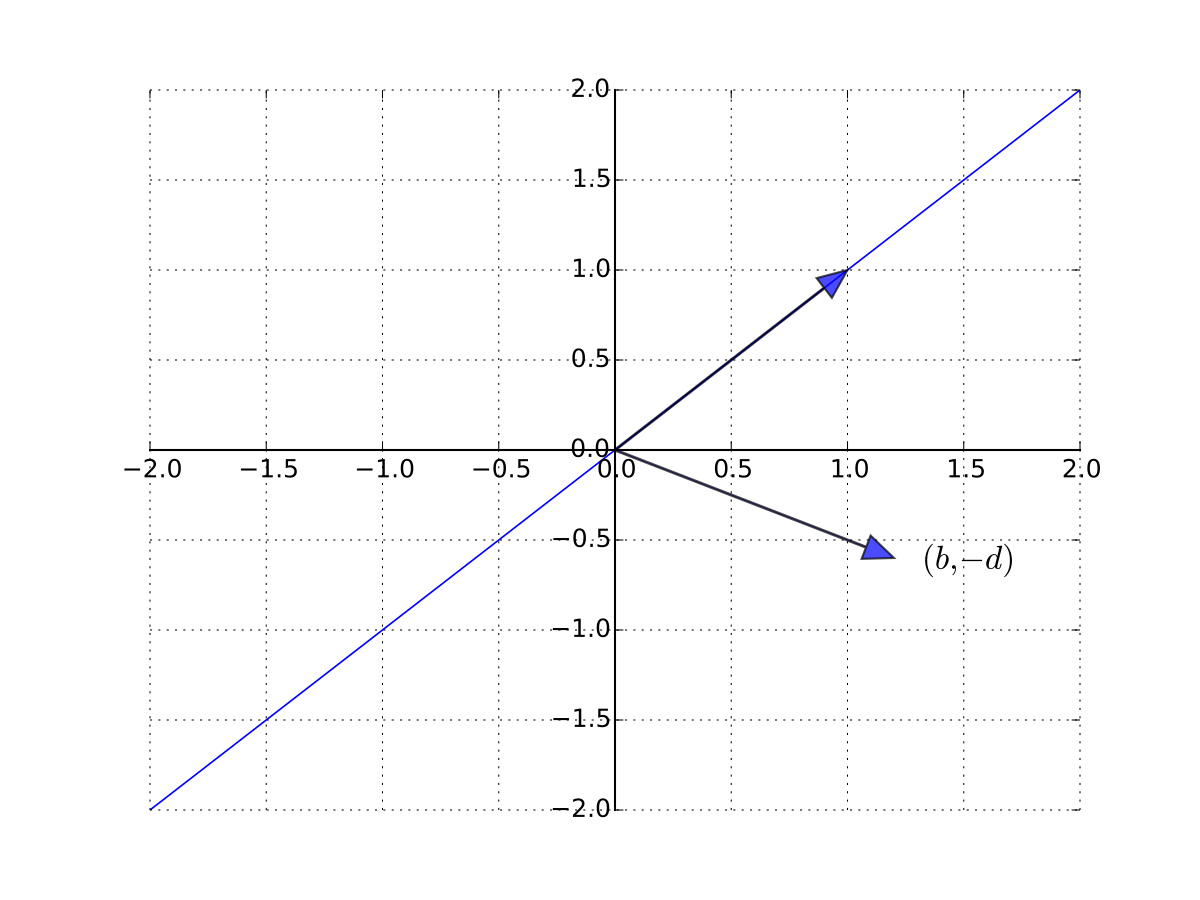
_images/not_multiple_of_one.png — Fig. 44 $(b, -d)$ is not a scalar multiple of $1$#

Example

Recall in the introduction we try to solve the system $A x = b$ of this form

\[\begin{split} A = \left[\begin{array}{cccc} 0 & 2 & 4 \\ 1 & 4 & 8 \\ 0 & 3 & 6 \\ \end{array} \right] \end{split}\]

The problem is that $A$ is singular (not nonsingular)

In particular, $\mathrm{col}_3(A) = 2 \mathrm{col}_2(A)$

Matrix inverse and inverse functions#

Definition

Given square matrix $A$, suppose $\exists$ square matrix $B$ such that

\[A B = B A = I\]

Then

$B$ is called the inverse of $A$, and written $A^{-1}$
$A$ is called invertible

Fact

A square matrix $A$ is nonsingular if and only if it is invertible

$A^{-1}$ is just the matrix corresponding to the linear mapping $T^{-1}$

Fact

Given nonsingular $n \times n$ matrix $A$ and $b \in \mathbb{R}^n$, the unique solution to $A x = b$ is given by

\[ x_b = A^{-1} b \]

Proof

Since $A$ is nonsingular we can immediately show that the solution is unique:

$T$ is a bijection, and hence one-to-one
if $A x = A y = b$ then $x = y$

To show that $x_b$ is indeed a solution we need to show that $A x_b = b$

To see this, observe that

\[ A x_b = A A^{-1} b = I b = b \]

Fact

In the $2 \times 2$ case, the inverse has the form

\[\begin{split} % \left( \begin{array}{cc} a & b \\ c & d \\ \end{array} \right)^{-1} = \frac{1}{ad - bc} \left( \begin{array}{cc} d & -b \\ -c & a \\ \end{array} \right) % \end{split}\]

Example

\[\begin{split} % A = \left( \begin{array}{cc} 1 & 2 \\ 1 & -1.5 \\ \end{array} \right) \quad \implies \quad A^{-1} = \frac{1}{-3.5} \left( \begin{array}{cc} -1.5 & -2 \\ -1 & 1 \\ \end{array} \right) % \end{split}\]

Fact

If $A$ is nonsingular and $\alpha \ne 0$, then

$A^{-1}$ is nonsingular and $(A^{-1})^{-1} = A$
$\alpha A$ is nonsingular and $(\alpha A)^{-1} = \alpha^{-1} A^{-1}$

Proof

Proof of part 2:

It suffices to show that $\alpha^{-1} A^{-1}$ is the right inverse of $\alpha A$

This is true because

\[ % \alpha A \alpha^{-1} A^{-1} = \alpha \alpha^{-1} A A^{-1} = I % \]

Fact

If $A$ and $B$ are $n \times n$ and nonsingular then

$A B$ is also nonsingular
$(A B)^{-1} = B^{-1} A^{-1}$

Proof

Let $T$ and $U$ be the linear mappings corresponding to $A$ and $B$

Recall that

$T \circ U$ is the linear mapping corresponding to $A B$
Compositions of linear mappings are linear
Compositions of bijections are bijections

Hence $T \circ U$ is a linear bijection with $(T \circ U)^{-1} = U^{-1} \circ T^{-1}$

That is, $AB$ is nonsingular with inverse $B^{-1} A^{-1}$

A different proof that $A B$ is nonsingular with inverse $B^{-1} A^{-1}$

Suffices to show that $B^{-1} A^{-1}$ is the right inverse of $A B$

To see this, observe that

\[ % A B B^{-1} A^{-1} = A A^{-1} = I % \]

Hence $B^{-1} A^{-1}$ is a right inverse as claimed

Singular case#

Example

The matrix $A$ with columns

\[\begin{split} % a_1 = \begin{pmatrix} 3 \\ 4 \\ 2 \end{pmatrix}, \quad a_2 = \begin{pmatrix} 3 \\ -4 \\ 1 \end{pmatrix} \quad \text{and} \quad a_3 = \begin{pmatrix} -3 \\ 4 \\ -1 \end{pmatrix} % \end{split}\]

is singular ($a_3 = - a_2$)

Its column space $\mathrm{span}(A)$ is just a plane in $\mathbb{R}^2$

Recall $b \in \mathrm{span}(A)$

$\iff$ $\exists \, x_1, \ldots, x_n$ such that $\sum_{k=1}^n x_j \mathrm{col}_j(A) = b$
$\iff$ $\exists \, x$ such that $A x = b$

Thus if $b$ is not in this plane then $A x = b$ has no solution

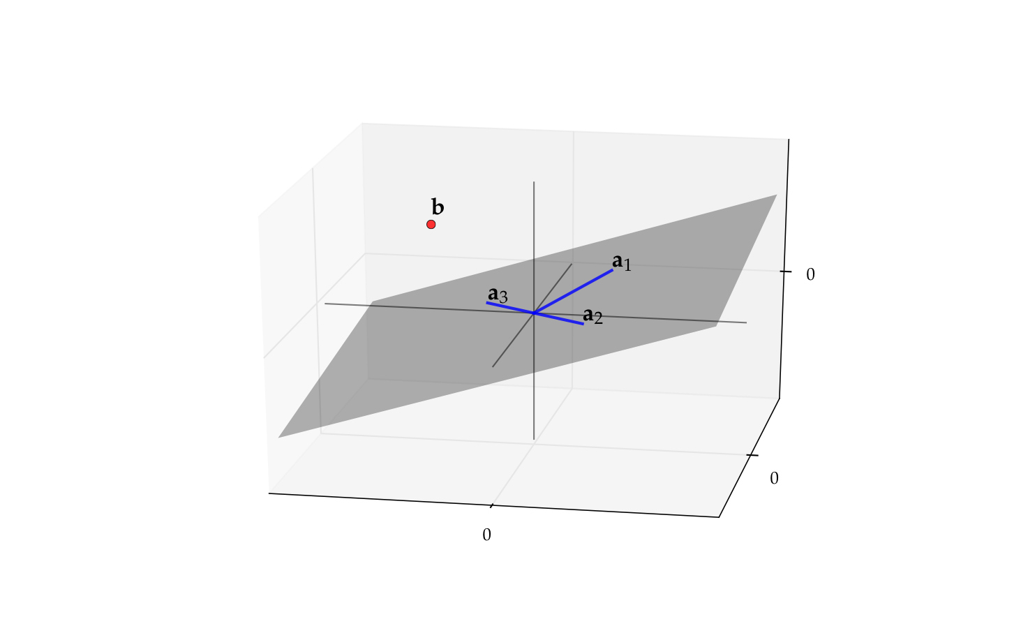
_images/not_in_span.png — Fig. 45 The vector $b$ is not in $\mathrm{span}(A)$#

Fact

If $A$ is a singular matrix and $A x = b$ has a solution then it has an infinity (in fact a continuum) of solutions

Proof

Let $A$ be singular and let $x$ be a solution

Since $A$ is singular there exists a nonzero $y$ with $A y = 0$

But then $\alpha y + x$ is also a solution for any $\alpha \in \mathbb{R}$ because

\[ % A(\alpha y + x) = \alpha A y + A x = A x = b % \]

Example

Back to the problem in the introduction where we try to solve the system $A x = b$ with

\[\begin{split} A = \left[\begin{array}{cccc} 0 & 2 & 4 \\ 1 & 4 & 8 \\ 0 & 3 & 6 \\ \end{array} \right], \quad b = \begin{pmatrix} 1 \\ 2 \\ 0 \end{pmatrix} \end{split}\]

As noted above we have $\mathrm{col}_3(A) = 2 \mathrm{col}_2(A)$, and therefore the matrix is singular.

Its column space is the

\[\begin{split} \mathrm{span}\left(\left\{ \begin{pmatrix} 0 \\ 1 \\ 0 \end{pmatrix}, \begin{pmatrix} 2 \\ 4 \\ 3 \end{pmatrix}, \begin{pmatrix} 4 \\ 8 \\ 6 \end{pmatrix} \right\}\right) = \mathrm{span}\left(\left\{ \begin{pmatrix} 0 \\ 1 \\ 0 \end{pmatrix}, \begin{pmatrix} 2 \\ 4 \\ 3 \end{pmatrix} \right\}\right) ,\end{split}\]

where we can drop the linearly dependent vector without changing the span.

Let’s see if the vector $b$ is in this span. We should look for $\alpha$ and $\beta$ such that

\[\begin{split} \begin{pmatrix} 1 \\ 2 \\ 0 \end{pmatrix} = \alpha \begin{pmatrix} 0 \\ 1 \\ 0 \end{pmatrix} + \beta \begin{pmatrix} 2 \\ 4 \\ 3 \end{pmatrix} \end{split}\]

From the first equation we have $\beta = 1/2$ while from the third $\beta=0$, thus this system does not have a solution in $(\alpha,\beta)$ and the vector $b$ is not in the span of the columns of $A$. We conclude that $Ax=b$ does not have solutions in this case.

But if $b$ was $(1,2,3/2)$ then we would conclude that $(\alpha,\beta) = (0,1/2)$ and thus $b$ would be in the span of the columns of $A$ even though they are linearly dependent. Then it is not hard to verify that any vector of the form $(0,0.5-2t,t)$ where $t \in \mathbb{R}$ is a free parameter, is a solution to the system. Note that there would be an infinity (continuum) of solutions in this case.

📖 Elements of linear algebra

Contents

📖 Elements of linear algebra#

Motivating example#

Vector Space#

Linear combinations#

Span#

Linear subspace#

Linear independence#

Bases and dimension#

Linear Functions#

Linearity and Bijections#

Mappings Across Different Dimensions#

Linear Functions are Matrix Multiplication#

Matrix Product as Composition#

Column Space#

Rank#

Systems of Linear Equations#

Matrix inverse and inverse functions#

Singular case#