Screencast of the lecture (part 1 and part 2)

📖 Unconstrained optimization

⏱ | words

References and additional materials

[Simon and Blume, 1994]

Chapters 17.1, 17.2, 17.3

[Sundaram, 1996]

Chapter 2.1, 2.2, 2.4, whole of chapter 4

A general optimization problem

Example

Consider a (monopolistic) firm that is facing a market demand for its products \(D(p) = \alpha + \frac{1}{4\alpha}p^2-p\) and the cost of production \(C(q) = \beta q + \delta q^2\). As usual, \(p\) and \(q\) denote price and quantity of product, respectively.

To maximize its profit \(\pi(p,q) = pq-C(q)\), the firm solves the following optimization problem

\[\begin{split} \Pi(\alpha,\beta,\delta) = \max_{p,q} \pi(p,q) = \max_{p,q} \big[ p q - C(q) \big] \\ \text {subject to} \\ q = D(p)\\ q \ge 0\\ p > 0 \end{split}\]

Plugging in the functions \(D(p)\) and \(C(q)\) we have an equivalent formulation

\[\begin{split} \Pi(\alpha,\beta,\delta) = \max_{p,q} \big[ (p-\beta) q - \delta q^2 \big] \\ \text {subject to} \\ q = \alpha + \frac{1}{4\alpha}p^2-p\\ q \ge 0\\ p > 0 \end{split}\]

Components of the optimization problem

1. Objective function: function to be maximized or minimized, also known as maximand
   In the example above profit function \(\pi(p,q) = pq - C(q)\) to be maximized

2. Decision/choice variables: the variables that the agent can control in order to optimize the objective function, also known as controls
   In the example above price \(p\) and quantity \(q\) variables that the firm can choose to maximize its profit

3. Equality constraints: restrictions on the choice variables in the form of equalities
   In the example above \(q = \alpha + \frac{1}{4\alpha}p^2-p\)

4. Inequality constraints (weak and strict): restrictions on the choice variables in the form of inequalities
   In the example above \(q \ge 0\) and \(p > 0\)

5. Parameters: the variables that are not controlled by the agent, but affect the objective function and/or constraints
   In the example above \(\alpha\), \(\beta\) and \(\delta\) are parameters of the problem

6. Value function: the “optimized” value of the objective function as a function of parameters
   In the example above \(\Pi(\alpha,\beta,\delta)\) is the value function

Definition

The general form of the optimization problem is

\[\begin{split} V(\theta) = \max_{x} f(x,\theta) \\ \text {subject to} \\ g_i(x,\theta) = 0, \; i\in\{1,\dots,I\}\\ h_j(x,\theta) \le 0, \; j\in\{1,\dots,J\} \end{split}\]

where:

• \(f(x,\theta) \colon \mathbb{R}^n \times \mathbb{R}^K \to \mathbb{R}\) is an objective function

• \(x \in \mathbb{R}^n\) are decision/choice variables

• \(\theta \in \mathbb{R}^K\) are parameters

• \(g_i(x,\theta) = 0, \; i\in\{1,\dots,I\}\) where \(g_i \colon \mathbb{R}^n \times \mathbb{R}^K \to \mathbb{R}\), are equality constraints

• \(h_j(x,\theta) \le 0, \; j\in\{1,\dots,J\}\) where \(h_j \colon \mathbb{R}^n \times \mathbb{R}^K \to \mathbb{R}\), are inequality constraints

• \(V(\theta) \colon \mathbb{R}^K \to \mathbb{R}\) is a value function

Definition

The set of admissible choices (admissible set) contains all the choices that satisfy the constraints of the optimization problem.

Note

Sometimes the equality constraints are dropped from the definition of the optimization problem, because they can always be represented as a pair of inequality constraints \(g_i(x,\theta) \le 0\) and \(-g_j(x,\theta) \le 0\)

Note

Note that strict inequality constraints are not present in the definition above, although they may be present in the economic applications. You already know that this has to do with the intention to keep the set of admissible choices closed, such that the solution of the problem (has a better chance to) exist. Sometimes they are added to the definition.

A roadmap for formulating an optimization problem (in economics)

1. Determine which variables are choice variables and which are parameters according to what the economic agent has control over

2. Determine whether the optimization problem is a maximization or a minimization problem

3. Determine the objective function of the economic agent (and thus the optimization problem)

4. Determine the constraints of the optimization problem: equality and inequality, paying particular attention to whether inequalities should be strict or weak (the latter has huge implications for the existence of the solution)

Example

Consider a decision maker who is deciding how to divide the money they have between food and services, bank deposit and buying some crypto. Discuss and Write down the corresponding optimization problem. [class exercise]

Classes of the optimization problems

1. Static optimization: finite number of choice variables

• singe instance of choice

• deterministic finite horizon dynamic choice models can be represented as static

• our main focus in this course

2. Dynamic programming: some choice variables are infinite sequences, solved using similar techniques as static optimization

• will touch upon in the end of the course

3. Deterministic optimal control: some “choice variables” are functions, completely new theory is needed

4. Stochastic optimal control: “choice variables” are functions, objective function is a stochastic process, yet more theory is needed

Reminder from one-dimensional optimization

Definition

Consider a function \(f: A \to \mathbb{R}\) where \(A \subset \mathbb{R}^n\). A point \(x^* \in A\) is called a

• maximizer of \(f\) on \(A\) if \(f(x^*) \geq f(x)\) for all \(x \in A\)

• minimizer of \(f\) on \(A\) if \(f(x^*) \leq f(x)\) for all \(x \in A\)

Definition

Point \(x \in \mathbb{R}\) is called interior to \([a, b]\) if \(a < x < b\)

A stationary point of \(f\) on \([a, b]\) is an interior point \(x\) with \(f'(x) = 0\)

Fact (first order condition)

If \(f\) is differentiable and \(x^*\) is either an interior minimizer or an interior maximizer of \(f\) on \([a, b]\), then \(x^*\) is stationary

\[ x^* \text{ is interior maximizer/minimizer } \implies x^* \text{ is stationary} \]

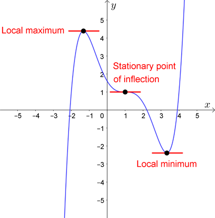
Fig. 55 Both \(x^*\) and \(x^{**}\) are stationary

Sufficient conditions for convexity/concavity in one dimension

Let \(f \colon [a, b] \to \mathbb{R}\)

• If \(f''(x) \geq 0\) for all \(x \in (a, b)\) then \(f\) is convex on \((a, b)\)

• If \(f''(x) > 0\) for all \(x \in (a, b)\) then \(f\) is strictly convex on \((a, b)\)

• If \(f''(x) \leq 0\) for all \(x \in (a, b)\) then \(f\) is concave on \((a, b)\)

• If \(f''(x) < 0\) for all \(x \in (a, b)\) then \(f\) is strictly concave on \((a, b)\)

Fact (shape conditions and uniqueness)

Let \(f \colon [a, b] \to \mathbb{R}\)

• If \(f\) is concave and \(x^* \in (a, b)\) is stationary then \(x^*\) is a maximizer

• If, in addition, \(f\) is strictly concave, then \(x^*\) is the unique maximizer

• If \(f\) is convex and \(x^* \in (a, b)\) is stationary then \(x^*\) is a minimizer

• If, in addition, \(f\) is strictly convex, then \(x^*\) is the unique minimizer

• We could also speak of second order conditions in the context of one-dimensional optimization, but we will cover them in the multivariate case below

Basic concepts in \(\mathbb{R}^n\)

In this lecture we focus on the unconstrained optimization problems of the form

\[ \max_{x} f(x,\theta), \qquad \min_{x} f(x,\theta) \]

which can also be written as

\[ f(x,\theta) \rightarrow \max, \qquad f(x,\theta) \rightarrow \min, \]

where \(f(x,\theta) \colon \mathbb{R}^n \to \mathbb{R}\) and unless stated otherwise is assumed to be continuous and twice continuously differentiable everywhere on \(\mathbb{R}^n\).

• Recall that twice continuously differentiable functions are referred to as \(C^2\)

• Parameter \(\theta\) may or may not be present.

• In \(\mathbb{R}\) we didn’t mention the destinction between constrained and non-constrained optimization

  • all examples were of constrained optimization problem with the constraint given by the domain of the function \([a,b]\)

  • in general constraints can be given in the definition of domain which is equivalent

  • In this lecture we focus on general functions \(f \colon \mathbb{R}^n \to \mathbb{R}\) without restrictions on their domain

• Every point in the whole space \(\mathbb{R}^n\) is interior, therefore we should expect that all maximizers/minimizers have to be stationary points

• Assuming differentiability implies we can focus on derivative based conditions

Definition

Given a function \(f \colon \mathbb{R}^n \to \mathbb{R}\), a point \(x \in \mathbb{R}^n\) is called a stationary point of \(f\) if \(\nabla f(x) = {\bf 0}\)

• Note gradient and zero vector \({\bf 0} = (0,\dots,0)\)

Only local maximizers/minimizers

• Recall that the approach for finding the global maximizers/minimizers of univariate functions was to compare the function values at all stationary points and the endpoints of the domain

  • this was sufficient to directly compare all points that could be maximizers/minimizers

  • crucially, the set of such points was finite

• In \(\mathbb{R}^n\) we can not have the same algorithm because the set of boundary points is in general infinite

  • lines/surfaces instead of endpoints

• Therefore, from now on focus only on local minimizers/maximizers

  • we will not be able to find the global maximizers/minimizers in general

Definition

Consider a function \(f: A \to \mathbb{R}\) where \(A \subset \mathbb{R}^n\). A point \(x^* \in A\) is called a

• local maximizer of \(f\) if \(\exists \delta>0\) such that \(f(x^*) \geq f(x)\) for all \(x \in B_\delta(x^*) \cap A\)

• local minimizer of \(f\) if \(\exists \delta>0\) such taht \(f(x^*) \leq f(x)\) for all \(x \in B_\delta(x^*) \cap A\)

If the inequality is strict, then \(x^\star\) is called a strict local maximizer/minimizer of \(f\)

• A global maximizer/minimizer must also be a local one, but the opposite is not true in general

First oder conditions (FOC)

• The first order conditions are the necessary conditions for a local maximizer/minimizer

Fact (Necessary condition for optima)

Let \(f(x,\theta) \colon \mathbb{R}^n \to \mathbb{R}\) be a differentiable function and let \(x^\star \in \mathbb{R}^n\) be a local maximizer/minimizer of \(f\). Then \(x^\star\) is a stationary point of \(f\), that is \(\nabla f(x^\star) = 0\)

\[ x^* \text{ is local maximizer/minimizer } \implies \nabla f(x^\star) = {\bf 0} \]

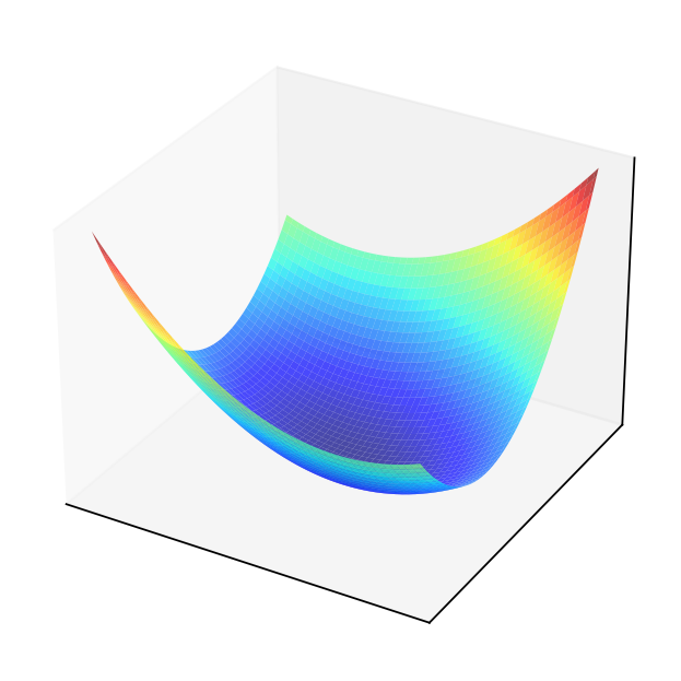
Example

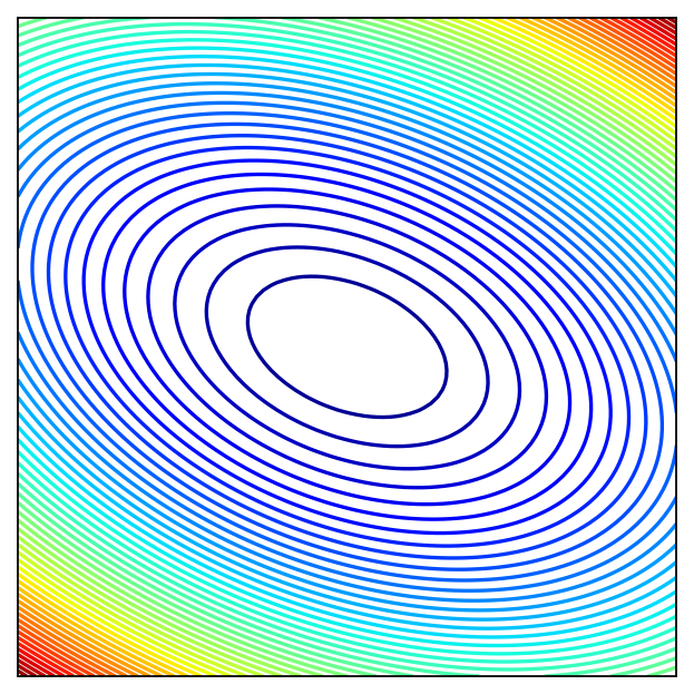
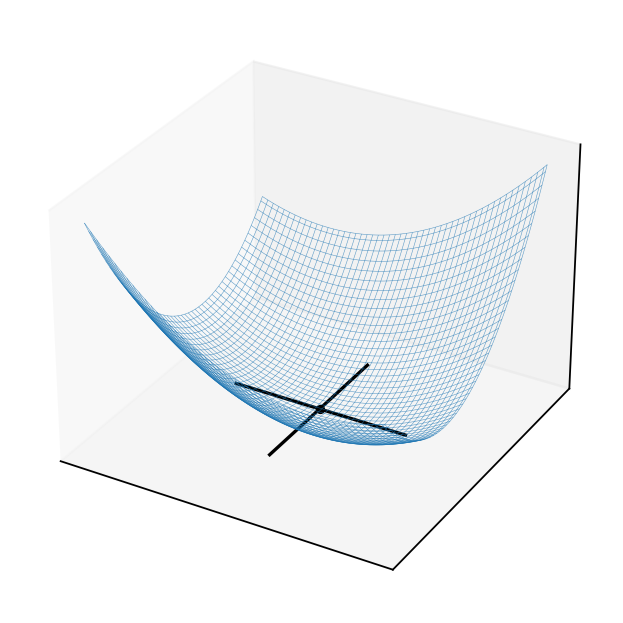
Consider quadratic form \(f(x) = x^T A x\) where \(A = \left( \begin{array}{rr} 1,& 0.5 \\ 0.5,& 2 \end{array} \right)\)

Solving the FOC

\[ \nabla f(x) = 2 x^T A = 0 \implies x = 0 \]

The point \((0,0)\) should be an optimizer.

Show code cell source Hide code cell source

import numpy as np
import matplotlib.pyplot as plt
from mpl_toolkits.mplot3d import Axes3D
from matplotlib import cm

A = np.array([[1,.5],[.5,2]])
f = lambda x: x@A@x
x = y = np.linspace(-5.0, 5.0, 100)
X, Y = np.meshgrid(x, y)
zs = np.array([f((x,y)) for x,y in zip(np.ravel(X), np.ravel(Y))])
Z = zs.reshape(X.shape)

fig = plt.figure(dpi=160)
ax1 = fig.add_subplot(111, projection='3d')
ax1.plot_surface(X, Y, Z, 
            rstride=2, 
            cstride=2,
            cmap=cm.jet,
            alpha=0.7,
            linewidth=0.25)
plt.setp(ax1,xticks=[],yticks=[],zticks=[])

fig = plt.figure(dpi=160)
ax2 = fig.add_subplot(111)
ax2.set_aspect('equal', 'box')
ax2.contour(X, Y, Z, 50,
            cmap=cm.jet)
plt.setp(ax2, xticks=[],yticks=[])

fig = plt.figure(dpi=160)
ax3 = fig.add_subplot(111, projection='3d')
ax3.plot_wireframe(X, Y, Z, 
            rstride=2, 
            cstride=2,
            alpha=0.7,
            linewidth=0.25)
f0 = f(np.zeros((2)))+0.1
ax3.scatter(0, 0, f0, c='black', marker='o', s=10)
ax3.plot([-3,3],[0,0],[f0,f0],color='black')
ax3.plot([0,0],[-3,3],[f0,f0],color='black')
plt.setp(ax3,xticks=[],yticks=[],zticks=[])

plt.show()

Example

Consider quadratic form \(f(x) = x^T A x\) where \(A = \left( \begin{array}{rr} 1,& 0.5 \\ 0.5,& -2 \end{array} \right)\)

Solving the FOC

\[ \nabla f(x) = 2 x^T A = 0 \implies x = 0 \]

The point \((0,0)\) should be an optimizer?

Show code cell source Hide code cell source

import numpy as np
import matplotlib.pyplot as plt
from mpl_toolkits.mplot3d import Axes3D
from matplotlib import cm

A = np.array([[1,.5],[.5,-2]])
f = lambda x: x@A@x
x = y = np.linspace(-5.0, 5.0, 100)
X, Y = np.meshgrid(x, y)
zs = np.array([f((x,y)) for x,y in zip(np.ravel(X), np.ravel(Y))])
Z = zs.reshape(X.shape)

fig = plt.figure(dpi=160)
ax1 = fig.add_subplot(111, projection='3d')
ax1.plot_surface(X, Y, Z, 
            rstride=2, 
            cstride=2,
            cmap=cm.jet,
            alpha=0.7,
            linewidth=0.25)
plt.setp(ax1,xticks=[],yticks=[],zticks=[])

fig = plt.figure(dpi=160)
ax2 = fig.add_subplot(111)
ax2.set_aspect('equal', 'box')
ax2.contour(X, Y, Z, 50,
            cmap=cm.jet)
plt.setp(ax2, xticks=[],yticks=[])

fig = plt.figure(dpi=160)
ax3 = fig.add_subplot(111, projection='3d')
ax3.plot_wireframe(X, Y, Z, 
            rstride=2, 
            cstride=2,
            alpha=0.7,
            linewidth=0.25)
f0 = f(np.zeros((2)))+0.1
ax3.scatter(0, 0, f0, c='black', marker='o', s=10)
ax3.plot([-3,3],[0,0],[f0,f0],color='black')
ax3.plot([0,0],[-3,3],[f0,f0],color='black')
plt.setp(ax3,xticks=[],yticks=[],zticks=[])

plt.show()

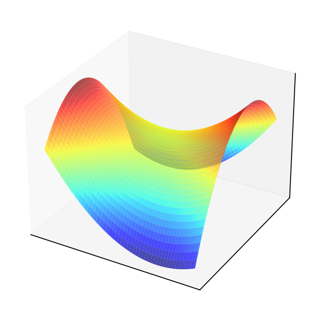
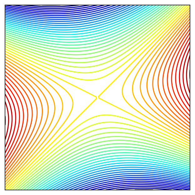
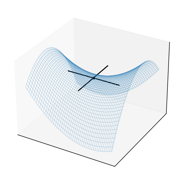
• This is an example of a saddle point where the FOC hold, yet the point is not a local maximizer/minimizer!

• Similar to \(x=0\) in \(f(x) = x^3\): derivative is zero, yet the point is not an optimizer

• How to distinguish saddle points from optima? Key insight: the second order derivative changes sign in this point

• In multivariate case the sign of the second derivative is equivalent to definiteness of the Hessian matrix!

Second order conditions (SOC)

• Allows us to establish whether the stationary point is a local maximizer/minimizer or a saddle point

• Help determining whether an optimizer is a maximizer or a minimizer

• But does not give definitive answer in all cases, unfortunately!

Fact (necessary SOC)

Let \(f(x) \colon \mathbb{R}^n \to \mathbb{R}\) be a twice continuously differentiable function and let \(x^\star \in \mathbb{R}^n\) be a local maximizer/minimizer of \(f\). Then:

• \(f\) has a local maximum at \(x^\star \implies Hf(x^\star)\) is negative semi-definite

• \(f\) has a local minimum at \(x^\star \implies Hf(x^\star)\) is positive semi-definite

• Recall the definition of semi-definiteness

• Note that the logical implication goes one way!

Fact (sufficient SOC)

Let \(f(x) \colon \mathbb{R}^n \to \mathbb{R}\) be a twice continuously differentiable function. Then:

• if \(x\) satisfies the first order condition and \(Hf(x^\star)\) is negative definite, then \(x^\star\) is a strict local maximum of \(f\)

\[ \nabla f(x^\star) = 0 \text{ and } Hf(x^\star) \text{ is negative definite } \implies x^\star \text{ is a strict local maximum} \]

• if \(x\) satisfies the first order condition and \(Hf(x^\star)\) is positive definite, then \(x^\star\) is a strict local minimum of \(f\)

\[ \nabla f(x^\star) = 0 \text{ and } Hf(x^\star) \text{ is positive definite } \implies x^\star \text{ is a strict local minimum} \]

• observe that SOC are only necessary in the “weak” form, but are sufficient in the “strong” form

• this leaves room for ambiguity when we can not arrive at a conclusion — particular stationary point may be a local maximum or minimum

• but we can rule out saddle points for sure, in this case neither semi-definiteness nor definiteness can be established, the Hessian is indefinite

Example

Consider a one dimensional function \(f(x) = (x-1)^2\), \(\nabla f(x)=2x-2\), \(Hf(x) = 2\).

Point \(x=1\) is a stationary point where FOC is satisfied.

Treating \(Hf(x)\) as \(1 \times 1\) matrix, we can see it is positive definite at \(x=1\) (\(y'[2]y = 2y^2 > 0\) for all \(y \ne 0\)), therefore \(x=1\) is a strict local minimum of \(f\).

Example

Consider a one dimensional function \(f(x) = x^2-1\), \(\nabla f(x)=2x\), \(Hf(x) = 2\).

Point \(x=0\) is a stationary point where FOC is satisfied.

Treating \(Hf(x)\) as \(1 \times 1\) matrix, we can see it is positive definite at \(x=0\) (\(y'[2]y = 2y^2 > 0\) for all \(y \ne 0\)), therefore \(x=0\) is a strict local minimum of \(f\).

Example

Consider a one dimensional function \(f(x) = (x-1)^4\), \(\nabla f(x)=4(x-1)^3\), \(Hf(x) = 12(x-1)^2\).

Point \(x=1\) is a stationary point where FOC is satisfied.

Treating \(Hf(x)\) as \(1 \times 1\) matrix, we can see it is positive semi-definite (and negative semi-definite) at \(x=1\) (\(y'[0]y = 0 \ge 0\) and \(y'[0]y = 0 \le 0\) for all \(y \in \mathbb{R}\)), therefore at \(x=1\) function \(f\) may have a local minimum. But may have a local maximum as well. No definite conclusion! (In reality it is a local and global minimum)

Example

Consider a one dimensional function \(f(x) = (x+1)^3\), \(\nabla f(x)=3(x+1)^2\), \(Hf(x) = 6(x+1)\).

Point \(x=-1\) is a stationary point where FOC is satisfied.

Treating \(Hf(x)\) as \(1 \times 1\) matrix, we can see it is positive semi-definite (and negative semi-definite) at \(x=-1\) (\(y'[0]y = 0 \ge 0\) and \(y'[0]y = 0 \le 0\) for all \(y \in \mathbb{R}\)), therefore at \(x=1\) function \(f\) may have a local minimum. But may have a local maximum as well. No definite conclusion! (In reality it is neither local minimum nor maximum)

Simplified definiteness of Hessian in \(\mathbb{R}^2\) special case

Recall the eigenvalue criterion of definiteness for a symmetric matrix \(A\):

• positive definite \(\iff\) all eigenvalues are strictly positive

• negative definite \(\iff\) all eigenvalues are strictly negative

• nonpositive definite \(\iff\) all eigenvalues are nonpositive

• nonnegative definite \(\iff\) all eigenvalues are nonnegative

• indefinite \(\iff\) there are both positive and negative eigenvalues

Let \(H\) be a \(2 \times 2\) matrix \(\to\) eigenvalues are roots of a quadratic equation

\[\begin{split} H = \left( \begin{array}{cc} a & b \\ c & d \\ \end{array} \right) \quad \implies \quad H - \lambda I = \left( \begin{array}{cc} a - \lambda & b \\ c & d - \lambda \end{array} \right) \end{split}\]

\[\begin{split} \implies \det(H - \lambda I) = (a - \lambda)(d - \lambda) - bc \\ = \lambda^2 - (a + d) \lambda + (ad - bc) \\ = \lambda^2 - \mathrm{trace}(H) \lambda + \det(H) \end{split}\]

Hence the the two eigenvalues \(\lambda_1\) and \(\lambda_2\) of \(H\) are given by the two roots of

\[ \lambda^2 - \mathrm{trace}(H) \lambda + \det(H) = 0 \]

From the Viets’s formulas for a quadratic polynomial we have

\[\begin{split} \lambda_1 + \lambda_2 = \mathrm{trace}(H) \\ \lambda_1 \lambda_2 = \mathrm{det}(H) \end{split}\]

Applying this result to a Hessian of a function \(f: \mathbb{R}^2 \to \mathbb{R}\) we have

Fact

Given a twice continuously differentiable function \(f: \mathbb{R}^2 \to \mathbb{R}\) and a stationary point \(x^\star: \; \nabla f(x^\star) = 0\), the second order conditions provide:

1. if \(\mathrm{det}(Hf(x^\star)) > 0\) and \(\mathrm{trace}(Hf(x^\star)) > 0\) \(\implies\)

   • \(\lambda_1 > 0\) and \(\lambda_2 > 0\),

   • \(Hf(x^\star)\) is positive definite,

   • \(f\) has a strict local minimum at \(x^\star\)

2. if \(\mathrm{det}(Hf(x^\star)) > 0\) and \(\mathrm{trace}(Hf(x^\star)) < 0\) \(\implies\)

   • \(\lambda_1 < 0\) and \(\lambda_2 < 0\),

   • \(Hf(x^\star)\) is negative definite,

   • \(f\) has a strict local maximum at \(x^\star\)

3. if \(\mathrm{det}(Hf(x^\star)) = 0\) and \(\mathrm{trace}(Hf(x^\star)) > 0\) \(\implies\)

   • \(\lambda_1 = 0\) and \(\lambda_2 > 0\),

   • \(Hf(x^\star)\) is positive semi-definite (nonnegative definite),

   • \(f\) may have a local minimum \(x^\star\)

   • undeceive!

4. if \(\mathrm{det}(Hf(x^\star)) = 0\) and \(\mathrm{trace}(Hf(x^\star)) < 0\) \(\implies\)

   • \(\lambda_1 = 0\) and \(\lambda_2 < 0\),

   • \(Hf(x^\star)\) is negative semi-definite (nonpositive definite),

   • \(f\) may have a local maximum \(x^\star\)

   • undeceive!

5. if \(\mathrm{det}(Hf(x^\star)) < 0\)

   • \(\lambda_1\) and \(\lambda_2\) have different signs,

   • \(Hf(x^\star)\) is indefinite,

   • \(x^\star\) is a saddle point of \(f\)

Example

Consider a two dimensional function \(f(x) = (x_1-1)^2 + x_1 x_2^2\)

\[\begin{split} \nabla f(x)=\big( 2(x_1-1) + x_2^2, \; 2 x_1 x_2 \big), \quad Hf(x)= \left( \begin{array}{ll} 2,& 2 x_2 \\ 2 x_2,& 2 x_1 \end{array} \right) \end{split}\]

Point \(x_1^\star=(1,0)\) is a stationary point where FOC is satisfied.

\[\begin{split} Hf(x^\star) = \left( \begin{array}{ll} 2,& 0 \\ 0,& 2 \end{array} \right), \quad \mathrm{det}(Hf(x^\star)) = 4 > 0, \quad \mathrm{trace}(Hf(x^\star)) = 4 > 0 \end{split}\]

Therefore at \(x_1^\star=(1,0)\) function \(f\) has a strict local minimum.

Point \(x_2^\star=(1+\tfrac{\sqrt{2}}{2},-\sqrt{2})\) is also a stationary point where FOC is satisfied.

\[\begin{split} Hf(x^\star) = \left( \begin{array}{ll} 2,& 2\sqrt{2} \\ 2\sqrt{2},& 2-\sqrt{2} \end{array} \right), \quad \mathrm{det}(Hf(x^\star)) = -4 - 2\sqrt{2} < 0 \end{split}\]

Therefore at \(x_2^\star=(1,0)\) function \(f\) has a saddle point.

Point \(x_3^\star=(1-\tfrac{\sqrt{2}}{2},\sqrt{2})\) is yet another stationary point where FOC is satisfied.

\[\begin{split} Hf(x^\star) = \left( \begin{array}{ll} 2,& -2\sqrt{2} \\ -2\sqrt{2},& 2+\sqrt{2} \end{array} \right), \quad \mathrm{det}(Hf(x^\star)) = 2\sqrt{2} -4 < 0 \end{split}\]

Therefore again, at \(x_3^\star=(1,0)\) function \(f\) has a saddle point.