📖 Eigenvalues and diagonalization

Online test 2 this week on Sunday, March 30 😬
- covers material from the last three weeks
  - Matrix arithmetics
  - Multivariate differentiation
  - Vector spaces and linear operators
  - Egienvectors and diagonalization
- DO NOT FORGET
  - postponed tests only when validated by ANU’s procedure
- On short answer question write exactly what is asked
  - Single word is one and only on word!
  - Check your spelling
Next two weeks are teaching break 🎉
- Good time to go over the material you struggle with, read the textbook and look through the extra material (3Blue1Brown videos)
- Semester continues on Monday, April 14
- However, I will be away
- The lecture will be face-to-face, taught by my PhD student and tutor Wending Liu
- The week after that is Easter, April 21 lecture will be recorded
- I will see you in person on April 28
Online test 3 is on Sunday, April 27 😬
- will cover material from the previous two weeks
  - Unconstrained optimization
  - Convexity and uniqueness
- DO NOT FORGET
  - postponed tests only when validated by ANU’s procedure
Stay tuned to course announcements on Wattle

📖 Eigenvalues and diagonalization#

⏱ | words

Euclidean Space#

We looked at vector spaces in the last lecture:

Linear combination
Span
Linear independence
Basis and dimension
Linear transformations

Now we add an additional component to the mix: dot/inner product $\implies$ Euclidean space

Definition

The Euclidean space is a pair $(V,\boldsymbol{\cdot})$ where $V$ is a vector space and “$\boldsymbol{\cdot}$” is a function from $V \times V$ to $\mathbb{R}$ that satisfies the following properties:

For all $u,v,w \in V$ and $\alpha, \beta \in \mathbb{R}$:

“$\boldsymbol{\cdot}$” is symmetric: $u \boldsymbol{\cdot} v = v \boldsymbol{\cdot} u$
“$\boldsymbol{\cdot}$” is linear: $(\alpha u + \beta v) \boldsymbol{\cdot} w = \alpha (u \boldsymbol{\cdot} w) + \beta v \boldsymbol{\cdot} w$
“$\boldsymbol{\cdot}$” is positive definite: $u \boldsymbol{\cdot} u \geq 0$ and $u \boldsymbol{\cdot} u = 0 \iff u = 0$

Thus, the difference between vector space and Euclidean space is the inclusion of an additional binary operation on the elements of the vector space.

Dot (inner) product#

The standard name for the additional operation is dot product or inner product
Sometimes Euclidean spaces are also referred to as dot product or inner product spaces

Definition

The dot product (inner product) of two vectors $x, y \in \mathbb{R}^n$ is

\[ % x \cdot y = x^T y = \sum_{i=1}^n x_i y_i % \]

the notation $\square^T$ is transposition operation which flips the vector from column-vector to row-vector to allow for standard matrix application to apply
alternative notation that you can come across is $\square^\prime$

We can verify that the following properties hold for the dot product (as required by the definition of Euclidean space):

Fact: Properties of dot product

For any $\alpha, \beta \in \mathbb{R}$ and any $x, y \in \mathbb{R}^n$, the following statements are true:

$x^T y = y^T x$
$(\alpha x)^T (\beta y) = \alpha \beta (x^T y)$
$x^T (y + z) = x^T y + x^T z$

Norm#

Dot product allows us to measure distance in the Euclidean space!

Definition

The (Euclidean) norm of $x \in \mathbb{R}^n$ is defined as

\[ % \| x \| = \sqrt{x^T x } = \left( \sum_{i=1}^n x_i^2 \right)^{1/2} % \]

As before

$\| x \|$ represents the ``length’’ of $x$
$\| x - y \|$ represents distance between $x$ and $y$

Fact

For any $\alpha \in \mathbb{R}$ and any $x, y \in \mathbb{R}^n$, the following statements are true:

$\| x \| \geq 0$ and $\| x \| = 0$ if and only if $x = 0$
$\| \alpha x \| = |\alpha| \| x \|$
$\| x + y \| \leq \| x \| + \| y \|$ (triangle inequality)
$| x^T y | \leq \| x \| \| y \|$ (Cauchy-Schwarz inequality)

Example

By default vectors are usually thought of as column-vectors:

\[\begin{split} x=\left(\begin{array}{c}1\\2\\0\\2\end{array}\right), \quad y=\left(\begin{array}{c}0\\2\\2\\1\end{array}\right), \end{split}\]

\[\begin{split} x \cdot y = x^T y = \Big(1,2,0,2\Big) \left(\begin{array}{c}0\\2\\2\\1\end{array}\right) = 2\cdot2 +2\cdot1 = 6 \end{split}\]

\[ \|x\| = \sqrt{1+4+4} = 3, \quad \|y\| = \sqrt{4+4+1} = 3, \]

\[\begin{split} \|x+y\| = \left\| \left(\begin{array}{c}1\\4\\2\\3\end{array}\right) \right\| = \sqrt{1+16+4+9} = \sqrt{30} \end{split}\]

Triangle inequality:

\[ (3+3)^2 > 30 \; \implies \; \|x\|+\|y\| > \|x+y\| \]

Cauchy-Schwarz inequality:

\[ |x \cdot y| = 6 < 3 \cdot 3 = \|x\| \cdot \|y\| \]

Fact

Dot products of linear combinations satisfy

\[ % \left( \sum_{j=1}^{m_1} \alpha_j x_j \right)^T \left( \sum_{j=1}^{m_2} \beta_j y_j \right) = \sum_{j=1}^{m_1} \sum_{k=1}^{m_2} \alpha_j \beta_k x_j^T y_k % \]

Proof

Follows from the properties of the dot product after some simple algebra

Orthogonality#

Definition

Consider an Euclidean space $(V, \boldsymbol{\cdot})$. Two vectors $x, y \in V$ are called to as orthogonal if

\[ x \boldsymbol{\cdot}y = x^T y = 0 \]

based on the geometric interpretation of dot product as the product of vector norms by the cosine of the angle between them, we can see that orthogonality implies that the angle between the vectors is $90^{\circ}$

Example

The elements of canonical basis in $\mathbb{R}^n$ are orthogonal to each other (pairwise orthogonal).

Indeed, take any $e_i$, $e_j$, $i \ne j$, from the canonical basis. These are both vectors with mainly zeros, and a single 1 in the $i$-th and $j$-th positions, respectively. Applying the dot product definition, the resuls is obviously zero.

Fact

Fix $a \in \mathbb{R}^n$ and let $A = \{ x \in \mathbb{R}^n \colon a^T x = 0 \}$

The set $A$ is a linear subspace of $\mathbb{R}^n$

Proof

Let $x, y \in A$ and let $\alpha, \beta \in \mathbb{R}$

We must show that $z = \alpha x + \beta y \in A$

Equivalently, that $a^T z = 0$

True because

\[ % a^T z = a^T (\alpha x + \beta y) = \alpha a^T x + \beta a^T y = 0 + 0 = 0 % \]

$a$ is referred to as the normal to the $n-1$-dimensional hyperplane $A$

Example

In $\mathbb{R}^3$ let $a=(2,-1,5)$, then $A$ is given by an equation $2x - y + 5z = 0$ which is a plane in 3D space.

Orthonormal basis#

Definition

A set $\{x_1, x_2, \dots, x_m\}$ where $x_j \in \mathbb{R}^n$ is called orthogonal set if each pair of vectors in the set is orthogonal

\[ x_i \cdot x_j = 0 \quad \text{for all } i \ne j \]

Definition

Consider a Euclidean space $(V,\boldsymbol{\cdot})$.

Orthogonal basis on $(V,\boldsymbol{\cdot})$ is any basis on $V$ which is also an orthogonal set.

Orthonormal basis on $(V,\boldsymbol{\cdot})$ is any orthogonal basis on $V$ all vectors of which have unit norm.

Example

Canonical basis in $\mathbb{R}^n$ is an example of an orthonormal basis.

\[\begin{split} e_1 = \left( \begin{array}{c} 1 \\ 0 \\ \vdots \\ 0 \end{array} \right), \quad e_2 = \left( \begin{array}{c} 0 \\ 1 \\ \vdots \\ 0 \end{array} \right), \; \cdots, \; e_n = \left( \begin{array}{c} 0 \\ 0 \\ \vdots \\ 1 \end{array} \right) \end{split}\]

Clearly, the dot product between each two vectors is zero, and each vector has norm $\sqrt{0+\dots+0+1^2+0+\dots+0}=1$.

Example

Consider the set $\left\{ \left( \begin{array}{c} 1 \\ 2 \end{array} \right), \left( \begin{array}{c} -2 \\ 1 \end{array} \right) \right\}$. It’s easy to check that they are linearly independent and therefore form a basis in their span (which is $\mathbb{R}^2$).

The dot product of these two vectors is $1 \cdot (-2) + 2 \cdot 1 = 0$, hence they are orthogonal. But this is not a orthonormal basis because the vectors do not have unit norm.

We could normalize the vectors to get an orthonormal basis. First compute the norm of each:

\[\begin{split} \left\| \left( \begin{array}{c} 1 \\ 2 \end{array} \right) \right\| = \sqrt{1^2 + 2^2} = \sqrt{5} = \sqrt{1^2 + (-2)^2} = \left\| \left( \begin{array}{c} -2 \\ 1 \end{array} \right) \right\| \end{split}\]

Therefore the orthonormal basis “based on” the original set is

\[\begin{split} \left\{ \left( \begin{array}{c} 1/\sqrt{5} \\ 2/\sqrt{5} \end{array} \right), \left( \begin{array}{c} -2/\sqrt{5} \\ 1/\sqrt{5} \end{array} \right) \right\} \end{split}\]

Change of basis#

Coordinates of vector depend on the basis used to represent it
We can change the basis and thus the coordinates of the vector
This is like speaking different languages: the same vector can be represented by different coordinates
Let’s learn to translate between these languages!

Example

Think of number systems with different bases: the same number can be represented with different digit

\[ 28_{10} = 8 \cdot 1 + 2 \cdot 10 \]

\[ 11100_2 = 0 \cdot 1 + 0 \cdot 2 + 1 \cdot 4 + 1 \cdot 8 + 1 \cdot 16 = 4 + 8 + 16 = 28_{10} \]

\[ 1\mathrm{C}_{16} = C \cdot 1 + 1 \cdot 16 = 12_{10} + 16 = 28_{10} \]

Base of number syste $\leftrightarrow$ basis in vector space: not fundamental, just a convention

Consider a vector $x\in \mathbb{R}^n$ which has coordinates $(x_1,x_2,\dots,x_n)$ in canonical basis $(e_1,e_2,\dots,e_n)$, where $e_i = (0,\dots,0,1,0\dots,0)^T$

Definition

Coordinates of a vector are the coefficients of the linear combination of the basis vectors that is equal to the vector.

Recall (which fact?) that uniqueness of representation holds for any linear combinations, not only basis.

We have

\[ x = \sum_{i=1}^n x_i e_i \]

Consider a different basis in $\mathbb{R}^n$ denoted $(e'_1,e'_2,\dots,e'_n)$. By definition it must be a set of $n$ vectors that span the whole space (and are therefore linearly independent).

When writing $e'_i$ we imply that each $e'_i$ is written in the coordinates corresponding to the original basis $(e_1,e_2,\dots,e_n)$.

The coordinates of vector $x$ in basis $(e'_1,e'_2,\dots,e'_n)$ denoted $x' = (x'_1,x'_2,\dots,x'_n)$ are by definition

\[\begin{split} x = \sum_{i=1}^n x'_i e'_i = x'_1 \left( \begin{array}{c} \vdots \\ e'_1 \\ \vdots \end{array} \right) + \dots + x'_n \left( \begin{array}{c} \vdots \\ e'_n \\ \vdots \end{array} \right) = P x' \end{split}\]

Definition

The transformation matrix from basis $(e'_1,e'_2,\dots,e'_n)$ to the basis $(e_1,e_2,\dots,e_n)$ is composed of the coordinates of the vectors of the former basis in the latter basis, placed as columns:

\[\begin{split} P = \left( \begin{array}{cccc} \vdots & \vdots & & \vdots \\ e'_1, & e'_2, & \dots & e'_n \\ \vdots & \vdots & & \vdots \end{array} \right) \end{split}\]

$P$ translates new coordinates back to the existing coordinates (so that we can make sense what the vector is)

In other words, the same vector has coordinates $x = (x_1,x_2,\dots, x_n)$ in the original basis $(e_1,e_2,\dots,e_n)$ and $x' = (x'_1,x'_2,\dots, x'_n)$ in the new basis $(e'_1,e'_2,\dots,e'_n)$, and it holds

\[ x = P x', \quad x' = P^{-1} x \]

We now have a way to represent the same vector in different bases, i.e. change basis!

Example

\[\begin{split} \begin{array}{l} e'_1 = e_1 + e_2 \\ e'_2 = e_1 - e_2 \\ e'_3=e_3 \end{array} \implies P = \begin{pmatrix} 1 & 1 & 0 \\ 1 & -1 & 0 \\ 0 & 0 & 1 \end{pmatrix} \end{split}\]

The opposite transformation is possible due to the following fact.

Fact

The transformation matrix $P$ is nonsingular (invertible).

Proof

Because the transformation matrix maps a set of basis vectors to another set of basis vectors, they are linearly independent. By the properties of linear functions, $P$ is then non-singular, and $P^{-1}$ exists. $\blacksquare$

Linear functions in different bases#

Consider a linear map $A: x \mapsto Ax$ where $x \in \mathbb{R}^n$

Can we express the same linear map in a different basis?

Let $B$ be the matrix representing the same linear map in a new basis, where the transformation matrix is given by $P$.

\[ x \mapsto Ax \quad \iff \quad x' \mapsto Bx' \]

If the linear map is the same, can convert the argument to new basis, apply the $B$ transformation, and convert back to the orginal basis:

\[ Ax = P \big[ B (P^{-1}x) \big] = P B P^{-1}x \]

Definition

Square matrix $A$ is said to be similar to square matrix $B$ if there exist an invertible matrix $P$ such that $A = P B P^{-1}$.

Similar matrixes happen to be very useful when we can convert the linear map to a diagonal form which may be much easier to work with (see below)

Change to orthonormal basis#

Interesting things happen when we change basis to the orthonormal one.

Let $\{s_1,\dots,s_n\}$ be an orthonormal basis in $\mathbb{R}^n$. These vectors form columns of the transformation matrix $P$. Consider $P^TP$, and using the fact that $\{s_1,\dots,s_n\}$ is an orthogonal set of vectors with norm equal one, we have

\[\begin{split} P^T P = \left( \begin{array}{ccc} \dots & s_1 & \dots \\ \dots & s_2 & \dots \\ & \vdots & \\ \dots & s_n & \dots \\ \end{array} \right) \left( \begin{array}{cccc} \vdots & \vdots & & \vdots \\ s_1, & s_2, & \dots & s_n \\ \vdots & \vdots & & \vdots \end{array} \right)= \end{split}\]

\[\begin{split} = \left( \begin{array}{cccc} s_1 \boldsymbol{\cdot} s_1 & s_1 \boldsymbol{\cdot} s_2 & \dots & s_1 \boldsymbol{\cdot} s_n \\ s_2 \boldsymbol{\cdot} s_1 & s_2 \boldsymbol{\cdot} s_2 & \dots & s_2 \boldsymbol{\cdot} s_n \\ \vdots & \vdots & \ddots & \vdots \\ s_n \boldsymbol{\cdot} s_1 & s_n \boldsymbol{\cdot} s_2 & \dots & s_n \boldsymbol{\cdot} s_n \end{array} \right) = \left( \begin{array}{cccc} \|s_1\|^2 & 0 & \dots & 0 \\ 0 & \|s_2\|^2 & \dots & 0 \\ \vdots & \vdots & \ddots & \vdots \\ 0 & 0 & \dots & \|s_n\|^2 \end{array} \right) = I \end{split}\]

Definition

The matrix for which it holds

\[ P^T P = I \quad \iff \quad P^T = P^{-1} \]

is called orthogonal matrix.

The transformation matrix $P$ from the original basis to the orthonormal basis is an orthogonal matrix.

Example

Consider the previous example of the orthonormal basis

\[\begin{split} \left\{ \left( \begin{array}{c} 1/\sqrt{5} \\ 2/\sqrt{5} \end{array} \right), \left( \begin{array}{c} -2/\sqrt{5} \\ 1/\sqrt{5} \end{array} \right) \right\} \end{split}\]

The transformation matrix $P$ is

\[\begin{split} P = \left( \begin{array}{cc} 1/\sqrt{5} & -2/\sqrt{5}\\ 2/\sqrt{5} & 1/\sqrt{5} \end{array} \right) \end{split}\]

Let’s check if the transformation matrix $P$ is orthogonal:

\[\begin{split} P^TP = \left( \begin{array}{cc} 1/\sqrt{5} & 2/\sqrt{5}\\ -2/\sqrt{5} & 1/\sqrt{5} \end{array} \right) \left( \begin{array}{cc} 1/\sqrt{5} & -2/\sqrt{5}\\ 2/\sqrt{5} & 1/\sqrt{5} \end{array} \right) = \end{split}\]

\[\begin{split} = \left( \begin{array}{cc} 1/5 + 4/5 & -2/5+2/5\\ -2/5+2/5 & 4/5+1/5 \end{array} \right) = \left( \begin{array}{cc} 1 & 0 \\ 0 & 1 \end{array} \right) \end{split}\]

The implication of these facts is that the change of basis to the orthonormal one is particularly easy to perform: no need to invert the transformation matrix, just transpose it!

In other words, the same vector has coordinates $x = (x_1,x_2,\dots, x_n)$ in the original basis $(e_1,e_2,\dots,e_n)$ and $x' = (x'_1,x'_2,\dots, x'_n)$ in the new orthonormal basis $(e'_1,e'_2,\dots,e'_n)$, and it holds

\[ x = P x', \quad x' = P^T x \]

Let $A$ and $B$ be the matrixes representing the same linear map in the original and new orthonormal basis with the transformation matrix given by $P$.

\[ x \mapsto Ax \quad \iff \quad x' \mapsto Bx' \]

It holds

\[ Ax = P B P^T x \]

This explains the wide use of orthonormal basis in practice

Eigenvalues and Eigenvectors#

Let $A$ be a square matrix

Think of $A$ as representing a mapping $x \mapsto A x$, this is a linear function (see prev lecture)

But sometimes $x$ will only be scaled in the transformation:

\[ % A x = \lambda x \quad \text{for some scalar $\lambda$} % \]

Definition

If $A x = \lambda x$ holds and $x \ne {\bf 0}$, then

$x$ is called an eigenvector of $A$ and $\lambda$ is called an eigenvalue
$(x, \lambda)$ is called an eigenpair

Clearly $(x, \lambda)$ is an eigenpair of $A$ $\implies$ $(\alpha x, \lambda)$ is an eigenpair of $A$ for any nonzero $\alpha$, so infinitely many eigenvectors for each eigenvalue, forming infinitely many eigenpairs.

Example

Let

\[\begin{split} % A = \begin{pmatrix} 1 & -1 \\ 3 & 5 \end{pmatrix} % \end{split}\]

Then

\[\begin{split} % \lambda = 2 \quad \text{ and } \quad x = \begin{pmatrix} 1 \\ -1 \end{pmatrix} % \end{split}\]

form an eigenpair because $x \ne 0$ and

\[\begin{split} % A x = \begin{pmatrix} 1 & -1 \\ 3 & 5 \end{pmatrix} \begin{pmatrix} 1 \\ -1 \end{pmatrix} = \begin{pmatrix} 2 \\ -2 \end{pmatrix} = 2 \begin{pmatrix} 1 \\ -1 \end{pmatrix} = \lambda x % \end{split}\]

import numpy as np
A = [[1, 2],
     [2, 1]]
eigvals, eigvecs = np.linalg.eig(A)
for i in range(eigvals.size):
  x = eigvecs[:,i]
  lm = eigvals[i]
  print(f'Eigenpair {i}:\n{lm:.5f} --> {x}')
  print(f'Check Ax=lm*x: {np.dot(A, x)} = {lm * x}')

Eigenpair 0:
3.00000 --> [0.70710678 0.70710678]
Check Ax=lm*x: [2.12132034 2.12132034] = [2.12132034 2.12132034]
Eigenpair 1:
-1.00000 --> [-0.70710678  0.70710678]
Check Ax=lm*x: [ 0.70710678 -0.70710678] = [ 0.70710678 -0.70710678]

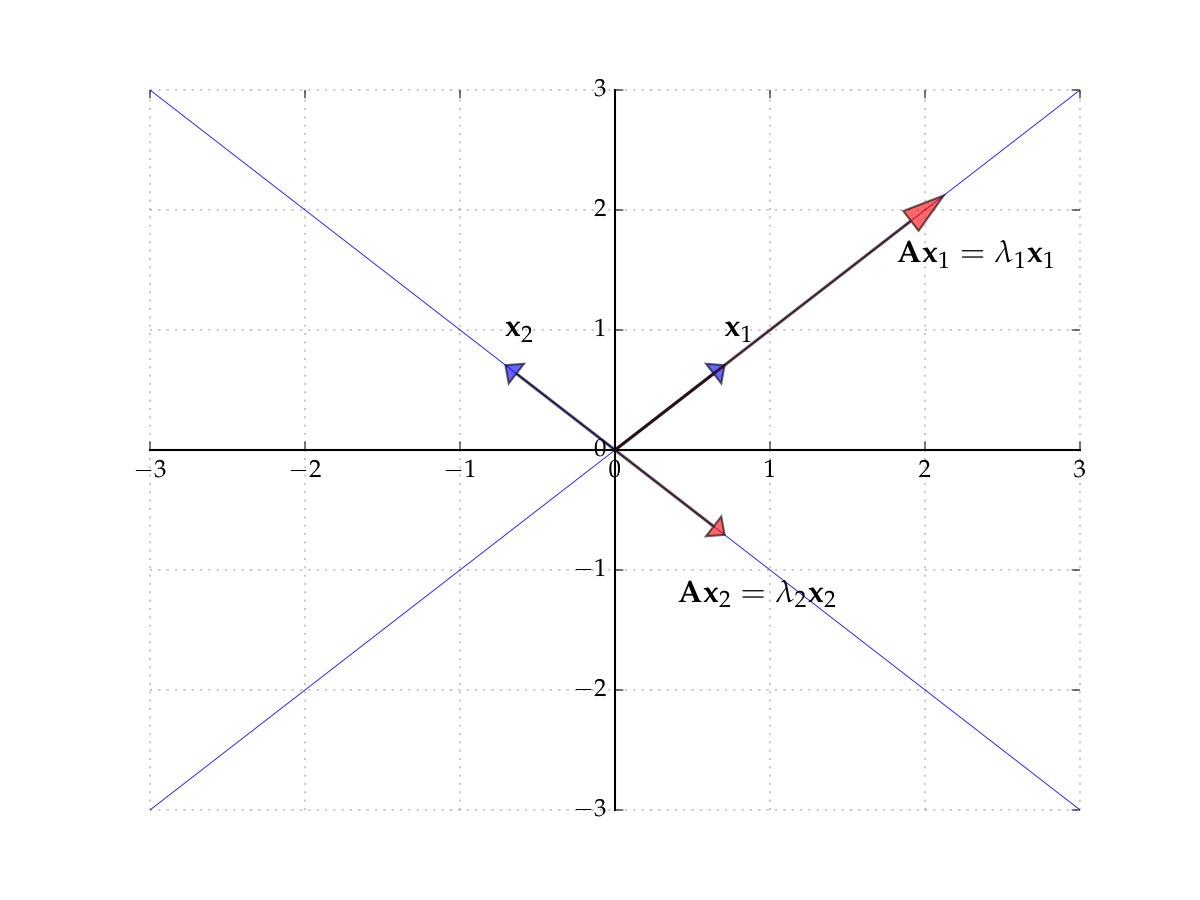
_images/eigenvecs.png — Fig. 46 The eigenvectors of $A$#

Consider the matrix

\[\begin{split} % R = \left( \begin{array}{cc} 0 & -1 \\ 1 & 0 \\ \end{array} \right) % \end{split}\]

Induces counter-clockwise rotation on any point by $90^{\circ}$

Hint

The columns of the matrix show where the classic basis vectors are translated to.

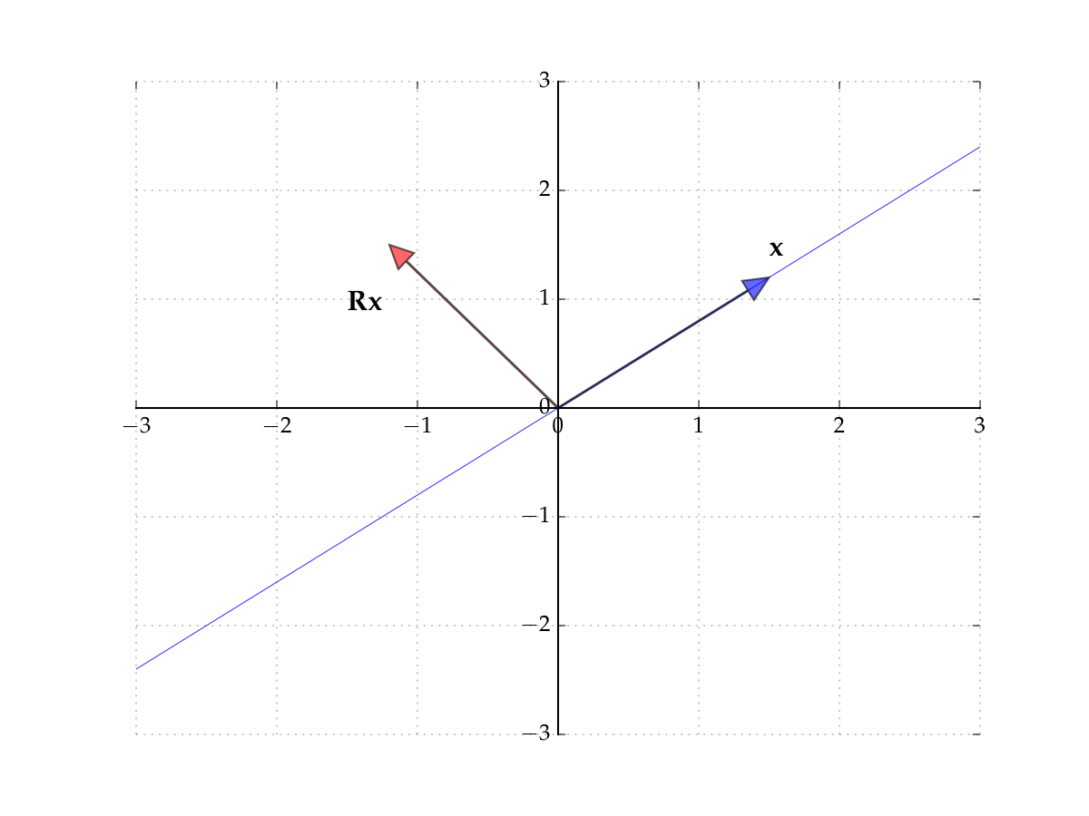
_images/rotation_1.png — Fig. 47 The matrix $R$ rotates points by $90^{\circ}$#

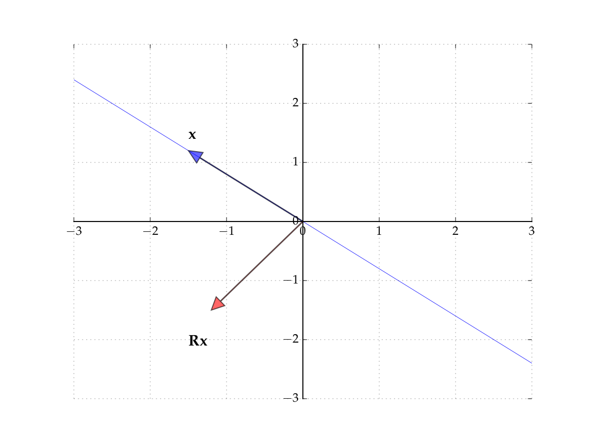
_images/rotation_2.png — Fig. 48 The matrix $R$ rotates points by $90^{\circ}$#

Hence no point $x$ is scaled

Hence there exists no pair $\lambda \in \mathbb{R}$ and $x \ne 0$ such that

\[R x = \lambda x\]

In other words, no real-valued eigenpairs exist. However, if we allow for complex values, then we can find eigenpairs even for this case as well.

Finding eigenvalues#

Fact

For any square matrix $A$

\[ % \lambda \text{ is an eigenvalue of } A \; \iff \; \det(A - \lambda I) = 0 % \]

Proof

Let $A$ by $n \times n$ and let $I$ be the $n \times n$ identity matrix

We have

\[\begin{split} \det(A - \lambda I) = 0 \iff A - \lambda I \text{ is singular} \\ \iff \text{null space (kernel) of } A - \lambda I \text{ is more than } \{0\} \\ \iff \exists \, x \ne 0 \text{ such that } (A - \lambda I) x = 0 \\ \iff \exists \, x \ne 0 \text{ such that } A x = \lambda x \\ \iff \lambda \text{ is an eigenvalue of } A \end{split}\]

Example

In the $2 \times 2$ case,

\[\begin{split} % A = \left( \begin{array}{cc} a & b \\ c & d \\ \end{array} \right) \quad \implies \quad A - \lambda I = \left( \begin{array}{cc} a - \lambda & b \\ c & d - \lambda \end{array} \right) % \end{split}\]

\[\begin{split} % \implies \det(A - \lambda I) = (a - \lambda)(d - \lambda) - bc \\ = \lambda^2 - (a + d) \lambda + (ad - bc) % \end{split}\]

Hence the eigenvalues of $A$ are given by the two roots of

\[ % \lambda^2 - (a + d) \lambda + (ad - bc) = 0 % \]

Equivalently,

\[ % \lambda^2 - \mathrm{trace}(A) \lambda + \det(A) = 0 % \]

Example

Consider the matrix

\[\begin{split} A = \left( \begin{array}{cc} 2 & 1 \\ 0 & 3 \end{array} \right) \end{split}\]

Note that $\mathrm{trace}(A)=5$ and $\det(A)=6$. The eigenvalues solve

\[ \lambda^2 - 5 \lambda + 6 = 0 \]

\[ \lambda_{1,2} = \frac{5 \pm \sqrt{5^2-4\cdot 6}}{2} = \frac{5 \pm 1}{2} = \{2, 3\} \]

Existence of Eigenvalues#

For an $(n \times n)$ matrix $A$ expression $\det(A - \lambda I) = 0$ is a polynomial equation of degree $n$ in $\lambda$

to see this, imagine how $\lambda$ enters into the computation of the determinant using the definition along the first row, then first row of the first minor submatrix, and so on
the highest degree of $\lambda$ is then the same as the dimension of $A$

Definition

The polynomial $\det(A - \lambda I)$ is called a characteristic polynomial of $A$.

The roots of the characteristic equation $\det(A - \lambda I) = 0$ determine all eigenvalues of $A$.

By the Fundamental theorem of algebra there are $n$ of such (complex) roots $\lambda_1, \ldots, \lambda_n$, and we can write

\[ % \det(A - \lambda I) = \prod_{j=1}^n (\lambda_j - \lambda) % \]

Each such $\lambda_i$ is an eigenvalue of $A$ because

\[ % \det(A - \lambda_i I) = \prod_{j=1}^n (\lambda_j - \lambda_i) = (\lambda_i-\lambda_i)\prod_{j \ne i} (\lambda_j - \lambda_i) = 0 % \]

not all roots are necessarily distinct — there can be repeats

Fact

By the fundamental theorem of algebra, every square $n \times n$ matrix has $n$ eigenvalues counted with (algebraic) multiplicity in the field of complex numbers $\mathbb{C}$.

So, there are two cases to be aware of:

eigenvalues with multiplicity greater than 1
eigenvalues that are not real numbers

Example

Consider the matrix

\[\begin{split} A = \left( \begin{array}{cc} 2 & 1 \\ 0 & 2 \end{array} \right) \end{split}\]

The characteristic polynomial is

\[\begin{split} \det(A - \lambda I) = \det \left( \begin{array}{cc} 2 -\lambda & 1 \\ 0 & 2-\lambda \end{array} \right) = (\lambda -2)^2 \end{split}\]

Therefore, both roots are $2$ and thus there is only eigenvalue. In this case we say that the eigenvalue has algebraic multiplicity 2.

Example

Consider the matrix

\[\begin{split} B = \left( \begin{array}{cc} 2 & 1 \\ -1 & 2 \end{array} \right) \end{split}\]

The characteristic polynomial is

\[\begin{split} \det(B - \lambda I) = \det \left( \begin{array}{cc} 2 -\lambda & 1 \\ -1 & 2-\lambda \end{array} \right) = (\lambda - 2)^2 +1 >0 \end{split}\]

Therefore, both roots are not real numbers. The eigenvalues are $\lambda = 2 \pm \sqrt{-1} \in \mathbb{C}$.

Fact

Characteristic polynomial $\det(A-\lambda I)$ does not change with the change of basis.

Proof

Let $B$ represent the same linear map as $A$ in the new basis, and let $P$ be a transformation matrix from the original basis to the new basis. We have $A = P B P^{-1}$.

Due to the properties of the determinant we have

\[ \det(A-\lambda I) = \det(P B P^{-1}-\lambda I) = \det(P B P^{-1}-\lambda P IP^{-1})= \]

\[ = \det\big(P (B -\lambda I)P^{-1}\big)= \det (P) \det (B -\lambda I) \det (P^{-1}) = \det (B -\lambda I) \]

$\blacksquare$

Fact

If $A$ is nonsingular, then eigenvalues of $A^{-1}$ are $1/\lambda_1, \ldots, 1/\lambda_n$

Proof

\[ A x = \lambda x \iff A^{-1}A x = \lambda A^{-1} x \iff x/\lambda = A^{-1} x \]

Finding eigenvectors from eigenvalues#

Once we know the eigenvalues, we may want to find eigenvectors that correspond to them.

Approach: plug the eigenvalue back into the equation $(A-\lambda I) x = 0$ and solve for $x$

we should not expect this system to have a single solution since $A-\lambda I$ is by definition singular
but we can recover a subspace of solutions that correspond to the given eigenvector
it is possible that multiple vectors correspond to the same eigenvalue

Example

We showed above that

\[\begin{split} A = \left( \begin{array}{cc} 2 & 1 \\ 0 & 3 \end{array} \right) \end{split}\]

has two distinct eigenvalues $\lambda_1 = 2$ and $\lambda_2 = 3$. Let’s find the eigenvectors corresponding to these eigenvalues.

\[\begin{split} \left( \begin{array}{cc|c} 2-2 & 1 & 0\\ 0 & 3-2 & 0 \end{array} \right) \to \left( \begin{array}{cc|c} 0 & 1 & 0\\ 0 & 1 & 0 \end{array} \right) \end{split}\]

The system places no restriction on $x_1$, and so any vector $(p,0)$ is a solution, $p$ is a free parameter. Therefore any vector of the form $(p,0)$ is an eigenvector corresponding to $\lambda_1 = 2$.

\[\begin{split} \left( \begin{array}{cc|c} 2-3 & 1 & 0\\ 0 & 3-3 & 0 \end{array} \right) \to \left( \begin{array}{cc|c} -1 & 1 & 0\\ 0 & 0 & 0 \end{array} \right) \end{split}\]

The system only requires $-x_1 + x_2 = 0$, that is $x_1=x_2$, therefore any vector of the form $(p,p)$ is a solution, and an eigenvector corresponding to $\lambda_2 = 3$.

Example

For the matrix

\[\begin{split} A = \left( \begin{array}{cc} 3 & 0 \\ 0 & 3 \end{array} \right) \end{split}\]

the characteristic polynomial is $(\lambda-3)^2$, and therefore there is one eigenvalues $\lambda = 3$ with multiplicity 2. Let’s find the eigenvectors corresponding to these eigenvalues.

\[\begin{split} \left( \begin{array}{cc|c} 3-3 & 0 & 0\\ 0 & 3-3 & 0 \end{array} \right) \to \left( \begin{array}{cc|c} 0 & 0 & 0\\ 0 & 0 & 0 \end{array} \right) \end{split}\]

The system places no restriction on either $x_1$ or $x_2$, and any vector $(x_1,x_2)$ is an eigenvector corresponding to $\lambda = 3$!

This is the case when it is possible to find a basis of two vectors in the linear subspace corresponding to the eigenvalue $\lambda = 3$, for example $(1,0)$ and $(0,1)$.

In this case we say that the eigenvalue has geometric multiplicity 2.

Geometrically, the linear transformation corresponding to the matrix $A$ stretches the space in both directions by the factor of 3.

Diagonalization#

Putting together eigenpairs and change of basis for the better good!

Diagonal matrixes#

Consider a square $n \times n$ matrix $A$

\[\begin{split} A = \left( \begin{array}{cccc} a_{11} & a_{12} & \cdots & a_{1n} \\ a_{21} & a_{22} & \cdots & a_{2n} \\ \vdots & \vdots & & \vdots \\ a_{n1} & a_{n2} & \cdots & a_{nn} \\ \end{array} \right) \end{split}\]

Definition

The $n$ elements of the form $a_{ii}$ are called the principal diagonal

Definition

A square matrix $D$ is called diagonal if all entries off the principal diagonal are zero

\[\begin{split} % D = \left( \begin{array}{cccc} d_1 & 0 & \cdots & 0 \\ 0 & d_2 & \cdots & 0 \\ \vdots & \vdots & & \vdots \\ 0 & 0 & \cdots & d_n \\ \end{array} \right) % \end{split}\]

Often written as

\[ % D = \mathrm{diag}(d_1, \ldots, d_n) % \]

Diagonal matrixes are very nice to work with!

Example

\[\begin{split} [\mathrm{diag}(d_1, \ldots, d_n) ]^2 = \left( \begin{array}{cccc} d_1 & 0 & \cdots & 0 \\ 0 & d_2 & \cdots & 0 \\ \vdots & \vdots & & \vdots \\ 0 & 0 & \cdots & d_n \\ \end{array} \right)^2 = \left( \begin{array}{cccc} d_1^2 & 0 & \cdots & 0 \\ 0 & d_2^2 & \cdots & 0 \\ \vdots & \vdots & & \vdots \\ 0 & 0 & \cdots & d_n^2 \\ \end{array} \right) = \mathrm{diag}(d_1^2, \ldots, d_n^2) \end{split}\]

Fact

If $D = \mathrm{diag}(d_1, \ldots,d_n)$ then

$D^k = \mathrm{diag}(d^k_1, \ldots, d^k_n)$ for any $k \in \mathbb{N}$
$d_n \geq 0$ for all $n$ $\implies$ $D^{1/2}$ exists and equals

\[\mathrm{diag}(\sqrt{d_1}, \ldots, \sqrt{d_n})\]

$d_n \ne 0$ for all $n$ $\implies$ $D$ is nonsingular and

\[D^{-1} = \mathrm{diag}(d_1^{-1}, \ldots, d_n^{-1})\]

Fact

The eigenvalues of a diagonal matrix are the diagonal elements themselves.

Proof

The characteristic polynomial is given by

\[\begin{split} \det(D-\lambda I) = \left| \begin{array}{cccc} d_1 - \lambda & 0 & \cdots & 0 \\ 0 & d_2 - \lambda & \cdots & 0 \\ \vdots & \vdots & & \vdots \\ 0 & 0 & \cdots & d_n - \lambda \\ \end{array} \right| = \Pi_{i=1}^n (d_i - \lambda) \end{split}\]

Therefore eigenvalues are $d_1, \ldots, d_n$, that is diagonal elements of the matrix.

$\blacksquare$

Concept of diagonalization#

recall that two matrices are similar if there is a change of basis transformation $P$ that connects the linear operators corresponding to these matrices such that $A = P D P^{-1}$

Definition

If $A$ is similar to a diagonal matrix, then $A$ is called diagonalizable

because diagonal matrices are easier to work with in many cases, diagonalization may be super useful in applications!

Example

Consider $A$ that is similar to a diagonal matrix $D = \mathrm{diag}(d_1,\dots,d_n)$.

To find the $A^n$ we can use the fact that

\[ A^2 = AA = P D P^{-1} P D P^{-1} = P D^2 P^{-1} \]

and therefore it’s easy to show by mathematical induction that

\[ A^k = AA^{k-1} = P D P^{-1} P D^{k-1} P^{-1} = P D^k P^{-1} \]

Given the properties of the diagonal matrixes, we have an easily computed expression

\[ A^k = P [\mathrm{diag}(d_1^k,\dots,d_n^k)] P^{-1} \]

Diagonalization using eigenpairs#

As you would anticipate, eigenvalues are most helpful in diagonalization

Fact (Diagonalizable $\longrightarrow$ Eigenpairs)

Let $n \times n$ matrix $A$ be diagonalizable with $A = P D P^{-1}$ and let

$D = \mathrm{diag}(\lambda_1, \ldots, \lambda_n)$
$p_j$ for $j=1,\dots,n$ be the columns of $P$

Then $(p_j, \lambda_j)$ is an eigenpair of $A$ for each $j \in \{1,\dots,n\}$

Proof

From $A = P D P^{-1}$ we get $A P = P D$

Equating $n$-th column on each side gives

\[ % A p_n = \lambda_n p_n % \]

Moreover $p_n \ne {\bf 0}$ because $P$ is invertible (otherwise determinant of $P$ would be zero).

Fact (Distinct eigenvalues $\longrightarrow$ diagonalizable)

If $n \times n$ matrix $A$ has $n$ distinct eigenvalues $\lambda_1, \ldots, \lambda_n$, then $A$ is diagonalizable with $A = P D P^{-1}$ where

$D = \mathrm{diag}(\lambda_1, \ldots, \lambda_n)$
each $n$-th column of $P$ is equal to an normlized eigenvector for $\lambda_n$

Example

Let

\[\begin{split} % A = \begin{pmatrix} 1 & -1 \\ 3 & 5 \end{pmatrix} % \end{split}\]

The eigenvalues of $A$ given by the equation

\[ \lambda^2 - 6 \lambda + 8 = 0 \]

are $\lambda_1=2$ and $\lambda_2=4$, while the eigenvectors are given by the solutions

\[\begin{split} \left( \begin{array}{cc|c} -1 & -1 & 0\\ 3 & 3 & 0 \end{array} \right) \to \left( \begin{array}{cc|c} 1 & 1 & 0\\ 0 & 0 & 0 \end{array} \right) \end{split}\]

\[\begin{split} \left( \begin{array}{cc|c} -3 & -1 & 0\\ 3 & 1 & 0 \end{array} \right) \to \left( \begin{array}{cc|c} 1 & 1/3 & 0\\ 0 & 0 & 0 \end{array} \right) \end{split}\]

as $(p,-p)$ and $(q,-3q)$ where $p$ and $q$ are free parameters. Imposing that the norm of the eigenvectors should be 1, we find that the normalized eigenvectors are

\[\begin{split} % p_1 = \begin{pmatrix} 1/\sqrt{2} \\ -1/\sqrt{2} \end{pmatrix} \quad \text{and} \quad p_2 = \begin{pmatrix} 1/\sqrt{10} \\ -3/\sqrt{10} \end{pmatrix} % \end{split}\]

Hence

\[\begin{split} A = P \cdot \mathrm{diag}(2, 4) \cdot P^{-1} = \begin{pmatrix} 1/\sqrt{2} & 1/\sqrt{10} \\ -1/\sqrt{2} & -3/\sqrt{10} \end{pmatrix} \begin{pmatrix} 2 & 0 \\ 0 & 4 \end{pmatrix} \begin{pmatrix} 1/\sqrt{2} & 1/\sqrt{10} \\ -1/\sqrt{2} & -3/\sqrt{10} \end{pmatrix}^{-1} \end{split}\]

import numpy as np
from numpy.linalg import inv
A = np.array([[1, -1],
              [3, 5]])
eigvals, eigvecs = np.linalg.eig(A)
D = np.diag(eigvals)
P = eigvecs
print('A =',A,sep='\n')
print('D =',D,sep='\n')
print('P =',P,sep='\n')
print('P^-1 =',inv(P),sep='\n')
print('P*D*P^-1 =',P@D@inv(P),sep='\n')

A =
[[ 1 -1]
 [ 3  5]]
D =
[[2. 0.]
 [0. 4.]]
P =
[[-0.70710678  0.31622777]
 [ 0.70710678 -0.9486833 ]]
P^-1 =
[[-2.12132034 -0.70710678]
 [-1.58113883 -1.58113883]]
P*D*P^-1 =
[[ 1. -1.]
 [ 3.  5.]]

Fact

Given $n \times n$ matrix $A$ with distinct eigenvalues $\lambda_1, \ldots, \lambda_n$ we have

$\det(A) = \prod_{j=1}^n \lambda_n$
$A$ is nonsingular $\iff$ all eigenvalues are nonzero

Proof

The first statement follows from the properties of the determinant of a product:

\[\begin{split} \det(A) = \det(P \mathrm{diag}(\lambda_1,\dots,\lambda_n) P^{-1}) =\\= \det(P) \det(\mathrm{diag}(\lambda_1,\dots,\lambda_n)) \det(P^{-1}) =\\= det(P) \prod_{j=1}^n \lambda_n (\det(P))^{-1} = \prod_{j=1}^n \lambda_n \end{split}\]

For the second statement: $A$ is nonsingular $\iff$ $\det(A) \ne 0$ $\iff$ $\prod_{j=1}^n \lambda_n \ne 0$ $\iff$ all $\lambda_n \ne 0$

Diagonalization of symmetric matrices#

Recall that a matrix $A$ is symmetric if $A = A^T$

Very special case when things work out much nicer!

Fact

Eigenvalues of a symmetric matrix are real numbers.

\[ A = A^T \implies \lambda_j \in \mathbb{R} \; \forall j \]

Proof

Complete proof requires complex analysis, but here is intuition for $2 \times 2$ case.

\[\begin{split} \det \left( \begin{array}{cc} a - \lambda & b \\ b & c - \lambda \end{array} \right)= (a-\lambda)(c-\lambda) - b^2 = \lambda^2 - (a+c) \lambda + ac - b^2 \end{split}\]

\[ \lambda_{1,2} = \frac{a+c \pm \sqrt{(a+c)^2 - 4(ac-b^2)}}{2} = \frac{a+c \pm \sqrt{(a-c)^2 + 4b^2}}{2} \]

The descriminant is nonnegative for any $a,b,c$, and therefore the roots are real numbers.

Fact

Eigenvectors $p_i$ of a symmetric matrix $A$ corresponding to distinct eigenvalues $\lambda_i$ are orthogonal.

\[ A = A^T, \lambda_i \ne \lambda_j \implies p_i \boldsymbol{\cdot} p_j =0 \]

Proof

Consider any $i \ne j$ eigenvalues and eigenvectors

\[ p_i \boldsymbol{\cdot} A p_j = \lambda_j (p_i \boldsymbol{\cdot} p_j) \]

On the other hand, with transposition of $1 \times 1$ “matrix” we have

\[\begin{split} p_i \boldsymbol{\cdot} A p_j = p_i^T A p_j = (p_i^T A p_j)^T = p_j^T A^T p_i =\\ p_j^T A p_i = p_j^T \lambda_i p_i = \lambda_j (p_i \boldsymbol{\cdot} p_j) \end{split}\]

Subtracting the two expressions gives

\[ 0 = (\lambda_i - \lambda_j) (p_i \boldsymbol{\cdot} p_j), \]

and since $\lambda_i - \lambda_j \ne 0$, we have $p_i \boldsymbol{\cdot} p_j = 0$

$\blacksquare$

Example

\[\begin{split} A= \left( \begin{array}{cc} 1 & 4 \\ 4 & 1 \end{array} \right) \end{split}\]

\[\begin{split} \det \left( \begin{array}{cc} 1-\lambda & 4 \\ 4 & 1-\lambda \end{array} \right) = (1-\lambda)^2 - 16 = 0 \end{split}\]

The eigenvalues are $\lambda_1 = -3$ and $\lambda_2 = 5$.

The assiciated eigenvectors are of the form $(p,-p)$ and $(q,q)$ where $p$ and $q$ are free parameters. We have

\[ (p,-p) \boldsymbol{\cdot} (q,q) = pq-pq = 0, \]

that is (all possible) eigenvectors are orthogonal.

This is now sufficient to conclude that when all eigenvalues of a symmetric matrix are distinct, it is possible to diagonalize the matrix using the eigenvectors in the transfomation matrix, and because they form an orthogonal set, it is possible to ensure that the transformation matrix is orthogonal $\to$ easier to work with

Algorithm:

Find eigenvalues $\lambda_1, \ldots, \lambda_n$ of $A$, assume they are all different (distinct)
For each $\lambda_i$ find the corresponding eigenvector $p_i$
Form the othonormal set of eigenvectors $p_1, \ldots, p_n$
Form the transformation matrix $P$ from these eigenvectors, it is orthogonal
Form the diagonal matrix $D$ with the eigenvalues on the diagonal
The matrix $A$ can be diagonalized as $A = P D P^T$

However, even though the case of repeated eigenvalues is more involved and requires more advanced techniques, the following fact still holds

Fact

For any symmetric matrix $A$, it is possible to form an orthonormal basis from its eigenvectors.

The symmetric matrix $A$ can be diagonalized by an orthogonal transformation matrix formed from these eigenvectors.

Proof

Intuition:

Distinct eigenvalues $\to$ complete set of eigenvalues to form the bases.
Even when eigenvalues are not distinct, each repeated eigenvalue corresponds to the subspace with dimension equal to the multiplicity of the eigenvalue $\to$ still possible to form a basis.
Orthogonality of eigenvectors $\to$ orthonormality of the basis.
It is always possible to normalize the basis vectors $\to$ transformation matrix is orthogonal.

The only practical issue is multiplicity of eigenvalues, in which case finding the required eigenvectors to form the orthonormal basis requires more careful work.

📖 Eigenvalues and diagonalization

Contents

📖 Eigenvalues and diagonalization#

Euclidean Space#

Dot (inner) product#

Norm#

Orthogonality#

Orthonormal basis#

Change of basis#

Linear functions in different bases#

Change to orthonormal basis#

Eigenvalues and Eigenvectors#

Finding eigenvalues#

Existence of Eigenvalues#

Finding eigenvectors from eigenvalues#

Diagonalization#

Diagonal matrixes#

Concept of diagonalization#

Diagonalization using eigenpairs#

Diagonalization of symmetric matrices#