Screencast of the lecture

📖 Convexity and uniqueness of optimizers

⏱ | words

References and additional materials

[Simon and Blume, 1994]

Chapters 17.4, 17.5

[Sundaram, 1996]

Chapter 7.1, 7.3.2, 7.4

In the last lecture we said that all the optimization theory applies to local maximizers/minimizers. This is true in general, but we have a special case where things are much simpler: when the objective function has a particular shape:

• Concave functions \(\rightarrow\) local maxima are global maxima

• Convex functions \(\rightarrow\) local minima are global minima

• Concavity/convexity \(\rightarrow\) first order conditions become sufficient for optimality

• Strict concavity/convexity \(\rightarrow\) uniqueness of the maximum/minimum

Convexity/concavity are referred to as shape conditions

• Convexity is a shape property for sets

• Convexity and concavity are shape properties for functions

Convex Sets

Definition

A set \(C \subset \mathbb{R}^K\) is called convex if

\[ % x, y \text{ in } C \text{ and } 0 \leq \lambda \leq 1 \; \implies \; \lambda x + (1 - \lambda) y \in C % \]

Convexity \(\iff\) line between any two points in \(C\) lies in \(C\)

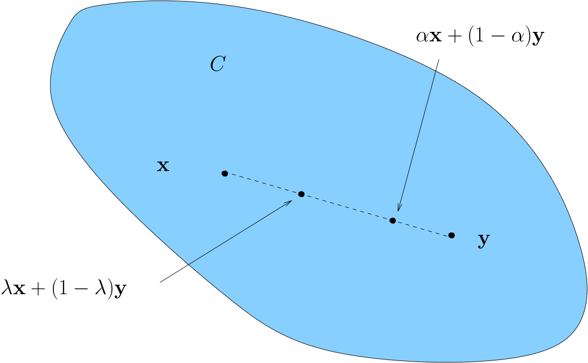
Fig. 56 Convex set

A non-convex set

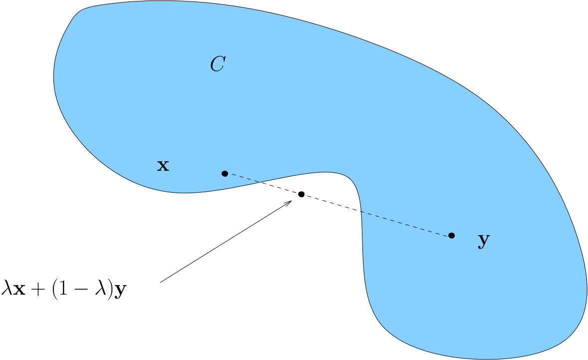
Fig. 57 Non-convex set

Example

The “positive cone” \(P := \{ x \in \mathbb{R}^K \colon x \geq 0 \}\) is convex

Proof

To see this, pick any \(x\), \(y\) in \(P\) and any \(\lambda \in [0, 1]\)

Let \(z := \lambda x + (1 - \lambda) y\) and let \(z_k := e_k' z\)

Since

• \(z_k = \lambda x_k + (1 - \lambda) y_k\)

• \(x_k \geq 0\) and \(y_k \geq 0\)

It is clear that \(z_k \geq 0\) for all \(k\)

Hence \(z \in P\) as claimed

Example

Every \(\epsilon\)-ball in \(\mathbb{R}^K\) is convex.

Proof

Fix \(a \in \mathbb{R}^K\), \(\epsilon > 0\) and let \(B_\epsilon(a)\) be the \(\epsilon\)-ball

Pick any \(x\), \(y\) in \(B_\epsilon(a)\) and any \(\lambda \in [0, 1]\)

The point \(\lambda x + (1 - \lambda) y\) lies in \(B_\epsilon(a)\) because

\[\begin{split} % \| \lambda x + (1 - \lambda) y - a \| = \| \lambda x - \lambda a + (1 - \lambda) y - (1 - \lambda) a \| \leq \\ \leq \| \lambda x - \lambda a \| + \| (1 - \lambda) y - (1 - \lambda) a \| = \\ = \lambda \| x - a \| + (1 - \lambda) \| y - a \| <> \\ < \lambda \epsilon + (1 - \lambda) \epsilon = \\ = \epsilon % \end{split}\]

Example

Let \(p \in \mathbb{R}^K\) and let \(M\) be the “half-space”

\[ % M := \{ x \in \mathbb{R}^K \colon p ' x \leq m\} % \]

The set \(M\) is convex

Proof

Let \(p\), \(m\) and \(M\) be as described

Fix \(x\), \(y\) in \(M\) and \(\lambda \in [0, 1]\)

Then \(\lambda x + (1 - \lambda) y \in M\) because

\[ % p'[\lambda x + (1 - \lambda) y ] = \lambda p'x + (1 - \lambda) p'y \leq \lambda m + (1 - \lambda) m = m % \]

Hence \(M\) is convex

Fact

If \(A\) and \(B\) are convex, then so is \(A \cap B\)

Proof

Let \(A\) and \(B\) be convex and let \(C := A \cap B\)

Pick any \(x\), \(y\) in \(C\) and any \(\lambda \in [0, 1]\)

Set

\[z := \lambda x + (1 - \lambda) y\]

Since \(x\) and \(y\) lie in \(A\) and \(A\) is convex we have \(z \in A\)

Since \(x\) and \(y\) lie in \(B\) and \(B\) is convex we have \(z \in B\)

Hence \(z \in A \cap B\)

Example

Let \(p \in \mathbb{R}^K\) be a vector of prices and consider the budget set

\[ % B(m) := \{ x \in \mathbb{R}^K \colon x \geq 0 \text{ and } p' x \leq m\} % \]

The budget set \(B(m)\) is convex

Proof

To see this, note that \(B(m) = P \cap M\) where

\[ % P := \{ x \in \mathbb{R}^K \colon x \geq 0 \} \qquad M := \{ x \in \mathbb{R}^K \colon p ' x \leq m\} % \]

We already know that

• \(P\) and \(M\) are convex, intersections of convex sets are convex

Hence \(B(m)\) is convex

Convex Functions

Let \(A \subset \mathbb{R}^K\) be a convex set and let \(f\) be a function from \(A\) to \(\mathbb{R}\)

Definition

\(f\) is called convex if

\[ % f(\lambda x + (1 - \lambda) y) \leq \lambda f(x) + (1 - \lambda) f(y) % \]

for all \(x, y \in A\) and all \(\lambda \in [0, 1]\)

\(f\) is called strictly convex if

\[ % f(\lambda x + (1 - \lambda) y) < \lambda f(x) + (1 - \lambda) f(y) % \]

for all \(x, y \in A\) with \(x \ne y\) and all \(\lambda \in (0, 1)\)

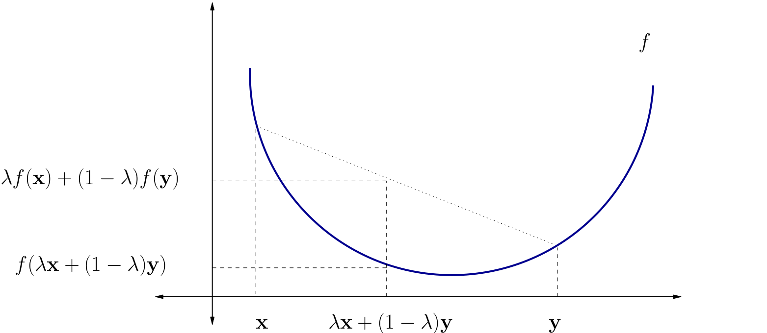
Fig. 58 A strictly convex function on a subset of \(\mathbb{R}\)

Fact

\(f \colon A \to \mathbb{R}\) is convex if and only if its epigraph (aka supergraph)

\[ E_f := \{ (x, y) \in A \times \mathbb{R} \colon f(x) \leq y \} \]

is a convex subset of \(\mathbb{R}^K \times \mathbb{R}\)

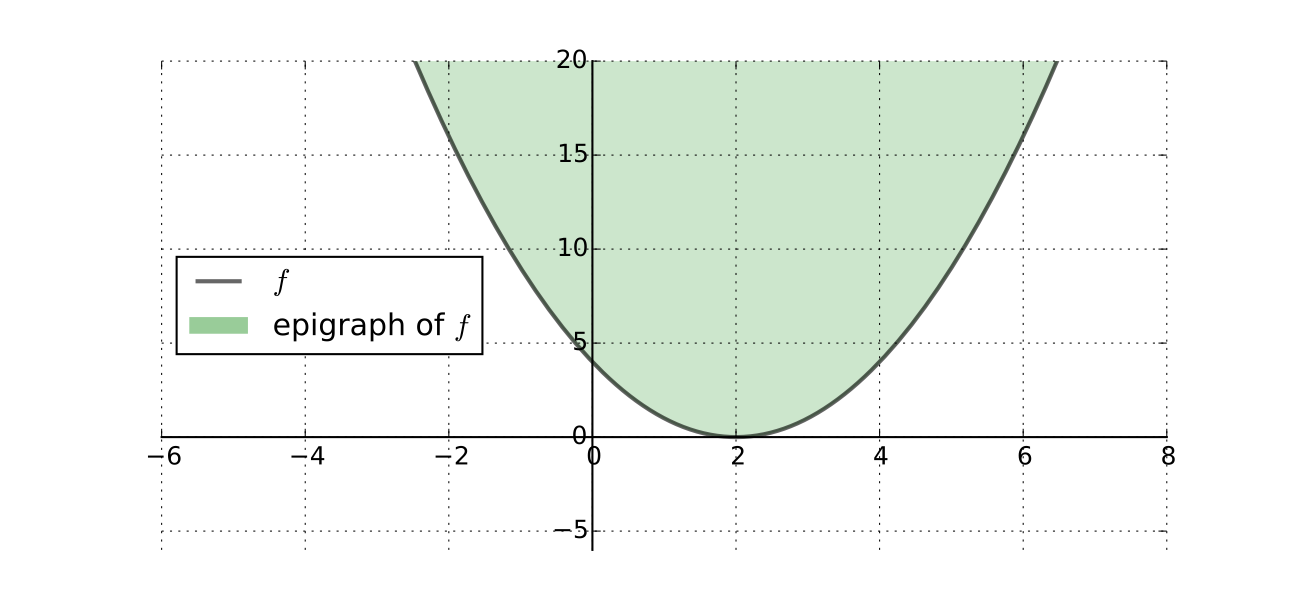
Fig. 59 Convex epigraph/supergraph of a function

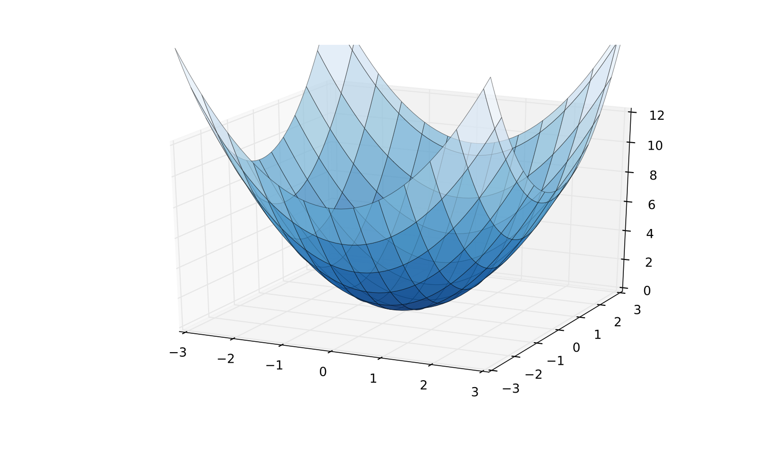
Fig. 60 A strictly convex function on a subset of \(\mathbb{R}^2\)

Example

\(f(x) = \|x\|\) is convex on \(\mathbb{R}^K\)

Proof

To see this recall that, by the properties of norms,

\[\begin{split} % \|\lambda x + (1 - \lambda) y\| \leq \|\lambda x\| + \|(1 - \lambda) y\| \\ = \lambda \|x\| + (1 - \lambda) \|y\| % \end{split}\]

That is,

\[ % f(\lambda x + (1 - \lambda) y) \leq \lambda f(x) + (1 - \lambda) f(y) % \]

Fact

If \(A\) is \(K \times K\) and positive definite, then

\[ Q(x) = x^T A x \qquad (x \in \mathbb{R}^K) \]

is strictly convex on \(\mathbb{R}^K\)

Proof

Proof: Fix \(x, y \in \mathbb{R}^K\) with \(x \ne y\) and \(\lambda \in (0, 1)\)

Exercise: Show that

\[\begin{split} % \lambda Q(x) + (1 - \lambda) Q(y) - Q(\lambda x + (1 - \lambda) y) \\ = \lambda (1 - \lambda) (x - y)' A (x - y) % \end{split}\]

Since \(x - y \ne 0\) and \(0 < \lambda < 1\), the right hand side is \(> 0\)

Hence

\[ % \lambda Q(x) + (1 - \lambda) Q(y) > Q(\lambda x + (1 - \lambda) y) % \]

Concave Functions

Let \(A \subset \mathbb{R}^K\) be a convex and let \(f\) be a function from \(A\) to \(\mathbb{R}\)

Definition

\(f\) is called concave if

\[ f(\lambda x + (1 - \lambda) y) \geq \lambda f(x) + (1 - \lambda) f(y) \]

for all \(x, y \in A\) and all \(\lambda \in [0, 1]\)

\(f\) is called strictly concave if

\[ f(\lambda x + (1 - \lambda) y) > \lambda f(x) + (1 - \lambda) f(y) \]

for all \(x, y \in A\) with \(x \ne y\) and all \(\lambda \in (0, 1)\)

Exercise: Show that

1. \(f\) is concave if and only if \(-f\) is convex

2. \(f\) is strictly concave if and only if \(-f\) is strictly convex

Fact

\(f \colon A \to \mathbb{R}\) is concave if and only if its hypograph (aka subgraph)

\[ % H_f := \{ (x, y) \in A \times \mathbb{R} \colon f(x) \geq y\} % \]

is a convex subset of \(\mathbb{R}^K \times \mathbb{R}\)

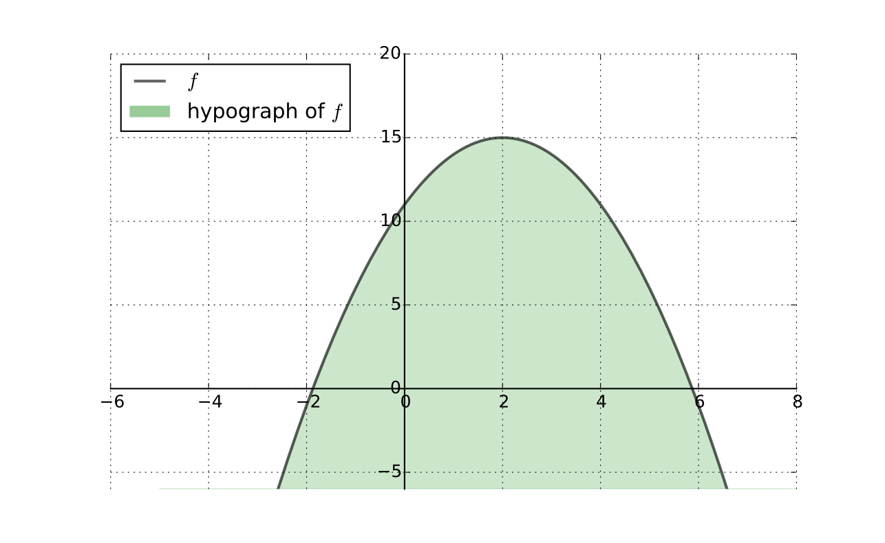
Fig. 61 Convex hypograph/subgraph of a function

Preservation of Shape

Let \(A \subset \mathbb{R}^K\) be convex and let \(f\) and \(g\) be functions from \(A\) to \(\mathbb{R}\)

Fact

If \(f\) and \(g\) are convex (resp., concave) and \(\alpha \geq 0\), then

• \(\alpha f\) is convex (resp., concave)

• \(f + g\) is convex (resp., concave)

If \(f\) and \(g\) are strictly convex (resp., strictly concave) and \(\alpha > 0\), then

• \(\alpha f\) is strictly convex (resp., strictly concave)

• \(f + g\) is strictly convex (resp., strictly concave)

Proof

Let’s prove that \(f\) and \(g\) convex \(\implies h := f + g\) convex

Pick any \(x, y \in A\) and \(\lambda \in [0, 1]\)

We have

\[\begin{split} % & h(\lambda x + (1 - \lambda) y) = f(\lambda x + (1 - \lambda) y) + g(\lambda x + (1 - \lambda) y) \\ & \leq \lambda f(x) + (1 - \lambda) f(y) + \lambda g(x) + (1 - \lambda) g(y) \\ & = \lambda [f(x) + g(x)] + (1 - \lambda) [f(y) + g(y)] \\ & = \lambda h(x) + (1 - \lambda) h(y) % \end{split}\]

Hence \(h\) is convex \(\blacksquare\)

Hessian based shape criterion

Fact

If \(f \colon A \to \mathbb{R}\) is a \(C^2\) function where \(A \subset \mathbb{R}^K\) is open and convex, then

1. \(Hf(x)\) positive semi-definite (nonnegative definite) for all \(x \in A\) \(\iff f\) convex

2. \(Hf(x)\) negative semi-definite (nonpositive definite) for all \(x \in A\) \(\iff f\) concave

In addition,

1. \(Hf(x)\) positive definite for all \(x \in A\) \(\implies f\) strictly convex

2. \(Hf(x)\) negative definite for all \(x \in A\) \(\implies f\) strictly concave

Proof: Omitted

Example

Let \(A := (0, \infty) \times (0, \infty)\) and let \(U \colon A \to \mathbb{R}\) be the utility function

\[ % U(c_1, c_2) = \alpha \ln c_1 + \beta \ln c_2 % \]

Assume that \(\alpha\) and \(\beta\) are both strictly positive

Exercise: Show that the Hessian at \(c := (c_1, c_2) \in A\) has the form

\[\begin{split} % H(c) := \begin{pmatrix} - \frac{\alpha}{c_1^2} & 0 \\ 0 & - \frac{\beta}{c_2^2} \end{pmatrix} % \end{split}\]

Exercise: Show that any diagonal matrix with strictly negative elements along the principle diagonal is negative definite

Conclude that \(U\) is strictly concave on \(A\)

Sufficiency of first order conditions

There two advantages of convexity/concavity:

1. Sufficiency of first order conditions for optimality

2. Uniqueness of optimizers with strict convexity/concavity

Fact (sufficient FOC)

Let \(A \subset \mathbb{R}^K\) be convex set and let \(f \colon A \to \mathbb{R}\) be concave/convex differentiable function. Then \(x^* \in A\) is a minimizer/minimizer of \(f\) on \(A\) if and only if \(x^*\) is a stationary point of \(f\) on \(A\).

\[ f \text{ concave } \implies \nabla f(x^*) = 0 \iff x^* \text{ is maximizer } \]

\[ f \text{ convex } \implies \nabla f(x^*) = 0 \iff x^* \text{ is minimizer } \]

• Note that weak convexity/concavity is enough for this result: first order condition becomes sufficient

• However, the optimizer may not be unique (see below results on uniqueness)

Proof

See [Sundaram, 1996], Theorem 7.15

Uniqueness of Optimizers

Fact

Let \(A \subset \mathbb{R}^K\) be convex set and let \(f \colon A \to \mathbb{R}\)

• If \(f\) is strictly convex, then \(f\) has at most one minimizer on \(A\)

• If \(f\) is strictly concave, then \(f\) has at most one maximizer on \(A\)

• with this fact we don’t know in general if \(f\) has a maximizer

• but if it does, then it has exactly one

Proof

Proof for the case where \(f\) is strictly concave:

Suppose to the contrary that

• \(a\) and \(b\) are distinct points in \(A\)

• both are maximizers of \(f\) on \(A\)

By the def of maximizers, \(f(a) \geq f(b)\) and \(f(b) \geq f(a)\)

Hence we have \(f(a) = f(b)\)

By strict concavity, then

\[ f\left( \frac{1}{2} a + \frac{1}{2} b \right) > \frac{1}{2} f( a) + \frac{1}{2} f( b) = \frac{1}{2} f( a) + \frac{1}{2} f( a) = f(a) \]

This contradicts the assumption that \(a\) is a maximizer

Fact (sufficient conditions for uniqueness)

Let \(A \subset \mathbb{R}^K\) be open convex set, let \(f \colon A \to \mathbb{R}\) be a \(C^2\) function, and \(x^* \in A\) stationary. Then if \(f\) strictly convex/concave, \(x^*\) is the unique minimizer/maximizer of \(f\) on \(A\).

2. \(f\) strictly convex \(\implies\) \(x^*\) is the unique minimizer of \(f\) on \(A\)

\[ f \text{ strictly concave } \implies \nabla f(x^*) = 0 \iff x^* \text{ is unique maximizer } \]

\[ f \text{ strictly convex } \implies \nabla f(x^*) = 0 \iff x^* \text{ is unique minimizer } \]

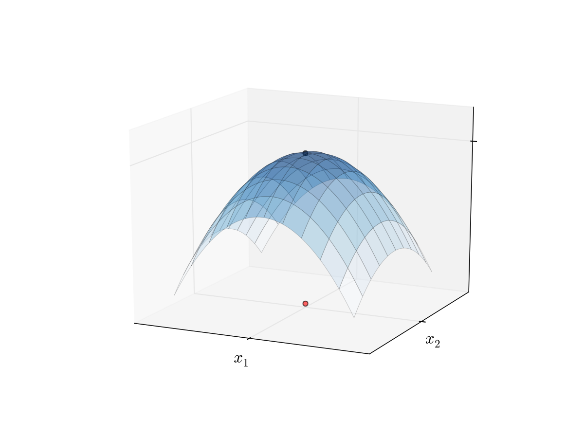
Fig. 62 Unique maximizer for a strictly concave function

Roadmap for unconstrained optimization

1. Assuming that the domain of the objective function is the whole space, check that the function is continuous and twice continuously differentiable to apply derivative based methods

2. Derive the gradient and Hessian of the objective function. Check if definiteness of Hessian can be established globally to show if shape conditions are satisfied.

3. Find all stationary points by solving FOC

4. If the function is (strictly) convex/concave, FOCs are sufficient for optimality. In the strict case, the stationary points are unique. Problem solved.

5. Otherwise, check SOC to determine whether found stationary points are local maxima or minima and filter out saddle points.

6. If asked to assess whether the identified local optima are global check the boundaries of the domain of the function, with the goal of comparing the function values there with those at the local optima. Also consider the limits of the function at infinity and check if there are any vertical asymptotes.

Example

\[ x^4+y^4+4xy \to \min \]

Let’s start by computing the gradient and Hessian of the function:

\[ \nabla f(x,y) = (4x^3+ 4y, 4y^3+4x) \]

\[\begin{split} Hf(x,y) = \begin{pmatrix} 12x^2 & 4 \\ 4 & 12y^2 \end{pmatrix} \end{split}\]

Is \(Hf(x,y)\) positive definite everywhere? The answer is given by the principal minors of the Hessian:

\[ D_{1,1} = 12x^2 > 0,\; D_{1,2} = 12y^2 > 0,\; D_{2} = 16\big(9x^2y^2-1\big) \]

It is obvious that \(D_2\) changes sign at the curve \(y=1/9x\), therefore the function is not convex or concave on \(\mathbb{R}^2\). We have to check both first and second order conditions.

\[\begin{split} \nabla f(x,y) = {\bf 0} \implies \begin{cases} x^3+y=0\\ x+y^3=0 \end{cases} \end{split}\]

By substituting \(y=-x^3\) into the second equation we have

\[\begin{split} -x^9+x = 0 \\ x(x^8-1) = 0 \\ x = 0 \text{ or } x = \pm 1 \end{split}\]

So, we have three stationary points, and examining the definiteness of the Hessian at them:

• \((0,0)\), \(D_2(0,0) <0\) \(\implies\) saddle point since the leading principal minors do not satisfy the definiteness pattern

• \((1,-1)\), \(D_2(1,-1) >0\) \(\implies\) \(Hf(1,-1)\) positive definite \(\implies\) local minimum

• \((-1,1)\), \(D_2(-1,1) >0\) \(\implies\) \(Hf(-1,1)\) positive definite \(\implies\) local minimum

Example

\[ x^4+y^4 \to \min \]

Let’s start by computing the gradient and Hessian of the function:

\[ \nabla f(x,y) = (4x^3, 4y^3) \]

\[\begin{split} Hf(x,y) = \begin{pmatrix} 12x^2 & 0 \\ 0 & 12y^2 \end{pmatrix} \end{split}\]

Clearly, the first and second leading principal minors are positive for all \(x,y \in \mathbb{R}\), therefore the function is strictly convex on \(\mathbb{R}^2\). We have to check first order conditions only which are in this case sufficient, and the minimizer is unique, both local and global.

\[\begin{split} \nabla f(x,y) = {\bf 0} \iff \begin{cases} x^3=0\\ y^3=0 \end{cases} \iff x=y=0. \end{split}\]