📖 Constrained optimization#
⏱ | words
WARNING
This section of the lecture notes is still under construction. It will be ready before the lecture.
Setting up a constrained optimization problem#
Let’s start with recalling the definition of a general optimization problem
Definition
The general form of the optimization problem is
where:
\(f(x,\theta) \colon \mathbb{R}^N \times \mathbb{R}^K \to \mathbb{R}\) is an objective function
\(x \in \mathbb{R}^N\) are decision/choice variables
\(\theta \in \mathbb{R}^K\) are parameters
\(g_i(x,\theta) = 0, \; i\in\{1,\dots,I\}\) where \(g_i \colon \mathbb{R}^N \times \mathbb{R}^K \to \mathbb{R}\), are equality constraints
\(h_j(x,\theta) \le 0, \; j\in\{1,\dots,J\}\) where \(h_j \colon \mathbb{R}^N \times \mathbb{R}^K \to \mathbb{R}\), are inequality constraints
\(V(\theta) \colon \mathbb{R}^K \to \mathbb{R}\) is a value function
Today we focus on the problem with constrants, i.e. \(I+J>0\)
The obvious classification that we follow
equality constrained problems, i.e. \(I>0\), \(J=0\)
inequality constrained problems, i.e. \(J>0\), which can include equalities as special case
Note
Note that every optimization problem can be seen as constrained if we define the objective function to have the domain that coincides with the admissible set.
is equivalent to
Constrained Optimization = economics#
A major focus of econ: the optimal allocation of scarce resources
optimal = optimization
scarce = constrained
Standard constrained problems:
Maximize utility given budget
Maximize portfolio return given risk constraints
Minimize cost given output requirement
Example
Maximization of utility subject to budget constraint
\(p_i\) is the price of good \(i\), assumed \(> 0\)
\(m\) is the budget, assumed \(> 0\)
\(x_i \geq 0\) for \(i = 1,2\)
let \(u(x_1, x_2) = \alpha \log(x_1) + \beta \log(x_2)\), \(\alpha>0\), \(\beta>0\)
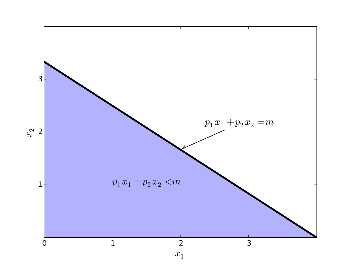
Fig. 63 Budget set when, \(p_1=0.8\), \(p_2 = 1.2\), \(m=4\)#
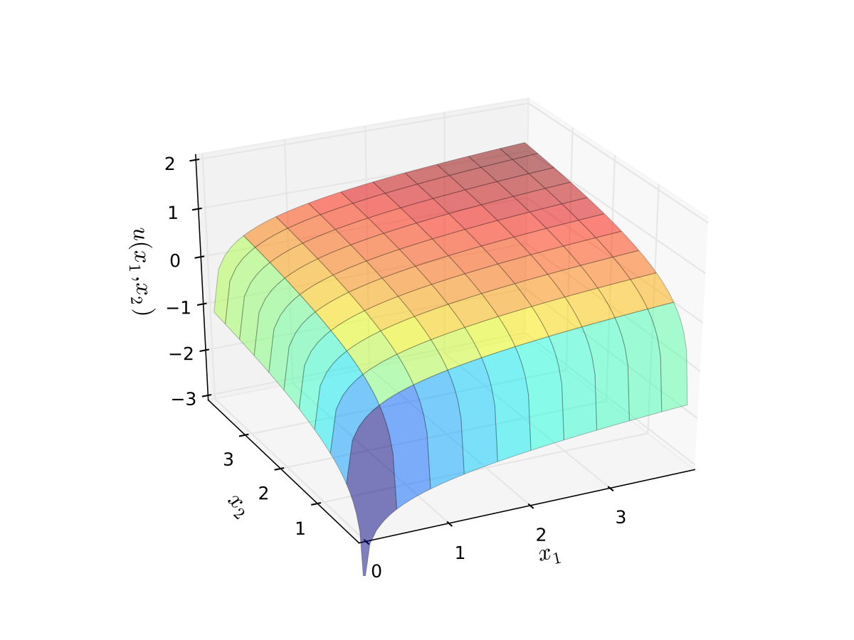
Fig. 64 Log utility with \(\alpha=0.4\), \(\beta=0.5\)#
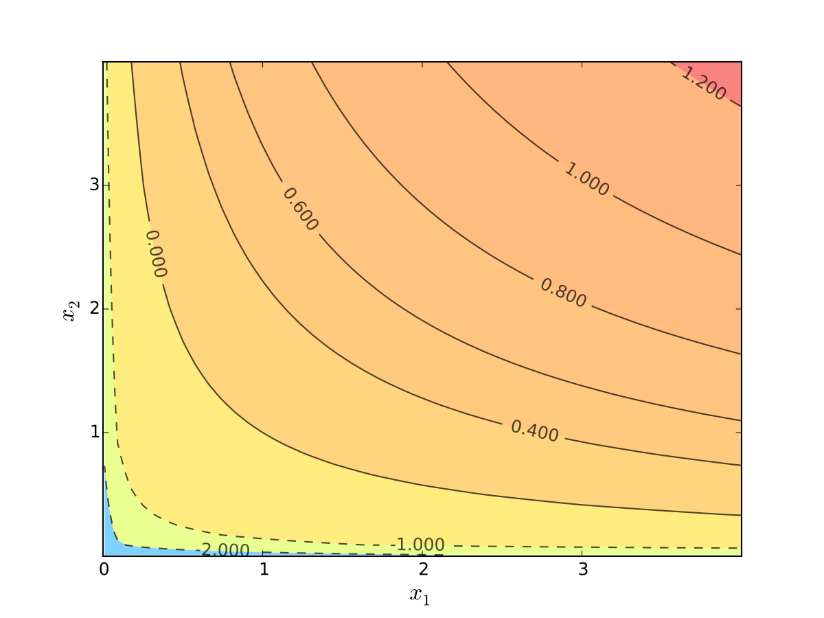
Fig. 65 Log utility with \(\alpha=0.4\), \(\beta=0.5\)#
We seek a bundle \((x_1^\star, x_2^\star)\) that maximizes \(u\) over the budget set
That is,
for all \((x_1, x_2)\) satisfying \(x_i \geq 0\) for each \(i\) and
Visually, here is the budget set and objective function:
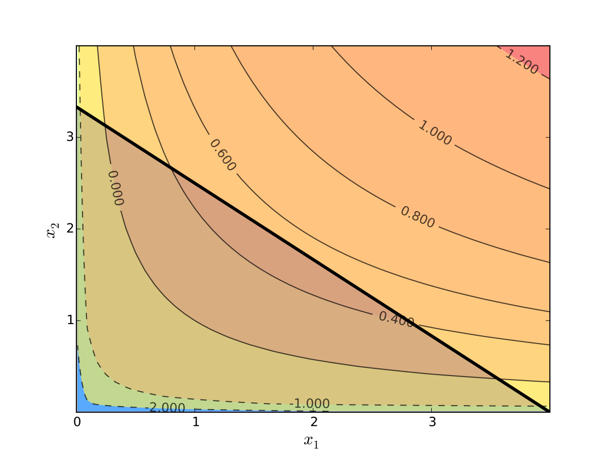
Fig. 66 Utility max for \(p_1=1\), \(p_2 = 1.2\), \(m=4\), \(\alpha=0.4\), \(\beta=0.5\)#
First observation: \(u(0, x_2) = u(x_1, 0) = u(0, 0) = -\infty\)
Hence we need consider only strictly positive bundles
Second observation: \(u(x_1, x_2)\) is strictly increasing in both \(x_i\)
Never choose a point \((x_1, x_2)\) with \(p_1 x_1 + p_2 x_2 < m\)
Otherwise can increase \(u(x_1, x_2)\) by small change
Hence we can replace \(\leq\) with \(=\) in the constraint
Implication: Just search along the budget line
Substitution Method#
Substitute constraint into objective function and treat the problem as unconstrained
This changes
into
Since all candidates satisfy \(x_1 > 0\) and \(x_2 > 0\), the domain is
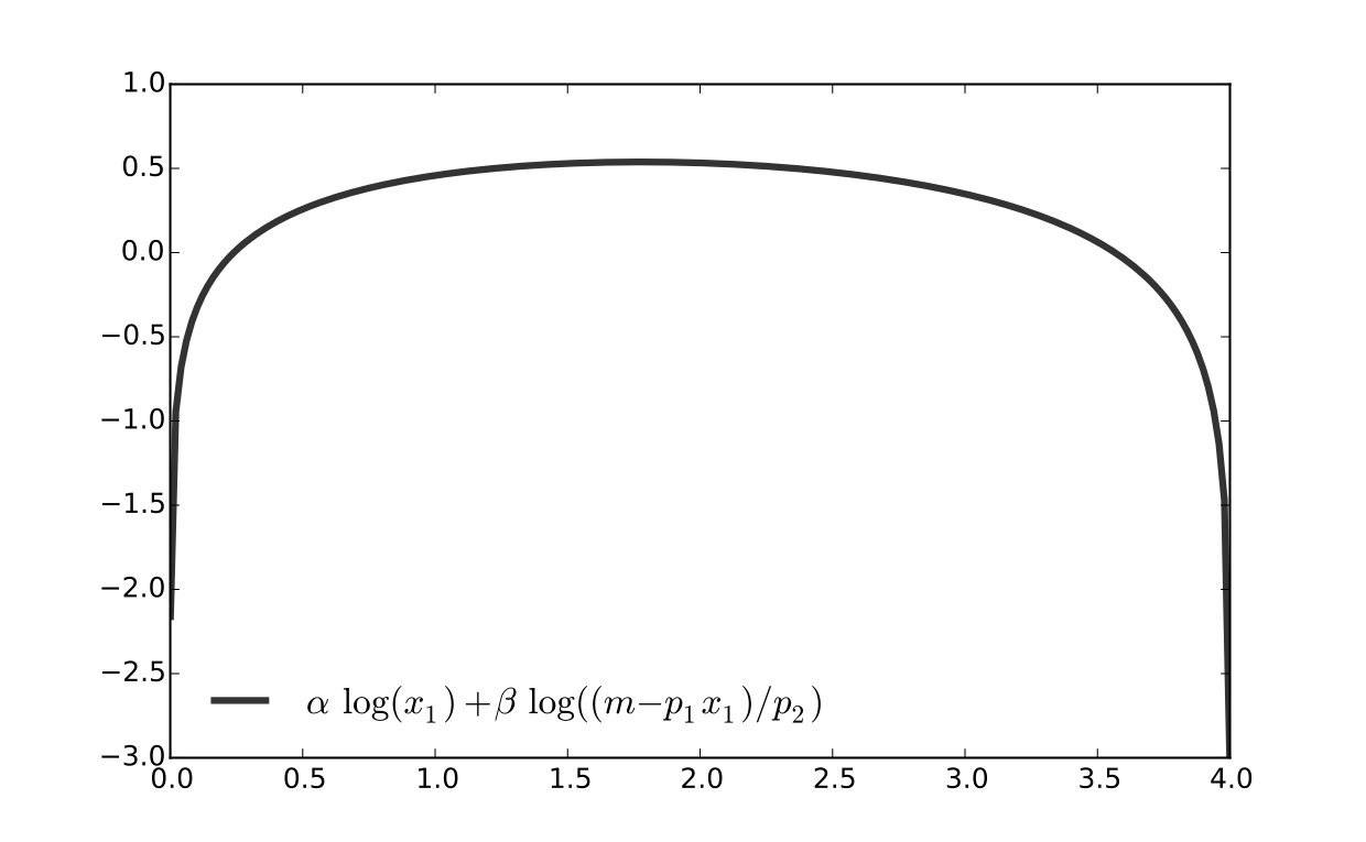
Fig. 67 Utility max for \(p_1=1\), \(p_2 = 1.2\), \(m=4\), \(\alpha=0.4\), \(\beta=0.5\)#
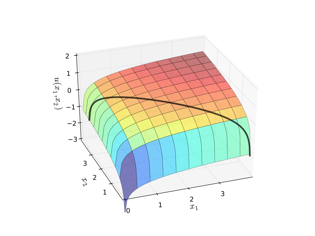
Fig. 68 Utility max for \(p_1=1\), \(p_2 = 1.2\), \(m=4\), \(\alpha=0.4\), \(\beta=0.5\)#
First order condition for
gives
Exercise: Verify
Exercise: Check second order condition (strict concavity)
Substituting into \(p_1 x_1^\star + p_2 x_2^\star = m\) gives
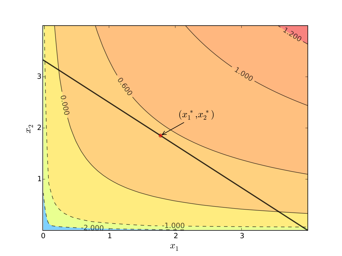
Fig. 69 Maximizer for \(p_1=1\), \(p_2 = 1.2\), \(m=4\), \(\alpha=0.4\), \(\beta=0.5\)#
Substitution method: algorithm#
How to solve
Steps:
Write constraint as \(x_2 = h(x_1)\) for some function \(h\)
Solve univariate problem \(\max_{x_1} f(x_1, h(x_1))\) to get \(x_1^\star\)
Plug \(x_1^\star\) into \(x_2 = h(x_1)\) to get \(x_2^\star\)
Limitations: substitution doesn’t always work
Example
Suppose that \(g(x_1, x_2) = x_1^2 + x_2^2 - 1\)
Step 1 from the cookbook says
use \(g(x_1, x_2) = 0\) to write \(x_2\) as a function of \(x_1\)
But \(x_2\) has two possible values for each \(x_1 \in (-1, 1)\)
In other words, \(x_2\) is not a well defined function of \(x_1\)
As we meet more complicated constraints such problems intensify
Constraint defines complex curve in \((x_1, x_2)\) space
Inequality constraints, etc.
We need more general, systematic approach
Tangency conditions#
Optimization approach based on tangency of contours and constraints
Example
Consider again the problem
Turns out that the maximizer has the following property:
budget line is tangent to an indifference curve at maximizer
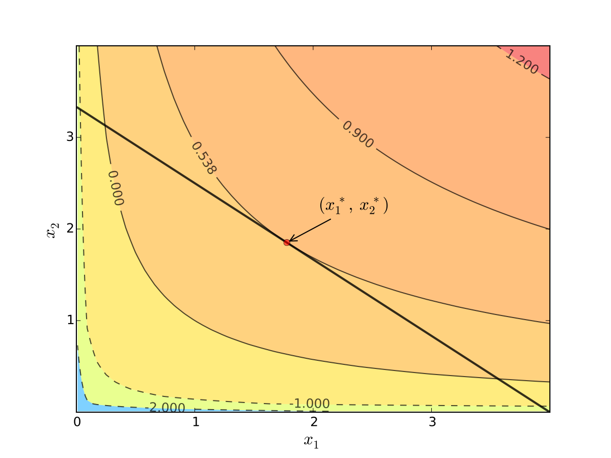
Fig. 70 Maximizer for \(p_1=1\), \(p_2 = 1.2\), \(m=4\), \(\alpha=0.4\), \(\beta=0.5\)#
In fact this is an instance of a general pattern
Notation: Let’s call \((x_1, x_2)\) interior to the budget line if \(x_i > 0\) for \(i=1,2\) (not a “corner” solution, see below)
In general, any interior maximizer \((x_1^\star, x_2^\star)\) of differentiable utility function \(u\) has the property: budget line is tangent to a contour line at \((x_1^\star, x_2^\star)\)
Otherwise we can do better:
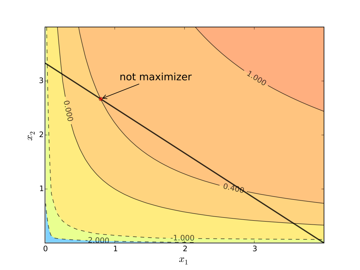
Fig. 71 When tangency fails we can do better#
Necessity of tangency often rules out a lot of points
We exploit this fact to build intuition and develop more general method
Relative Slope Conditions#
Consider an equality constrained optimization problem where objective and constraint functions are differentiable:
How to develop necessary conditions for optima via tangency?
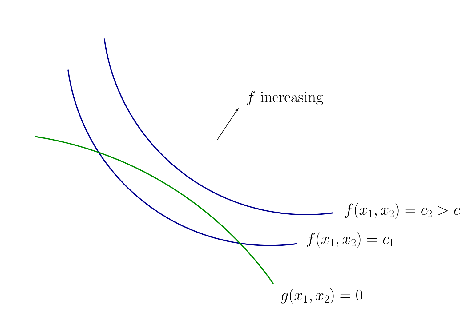
Fig. 72 Contours for \(f\) and \(g\)#
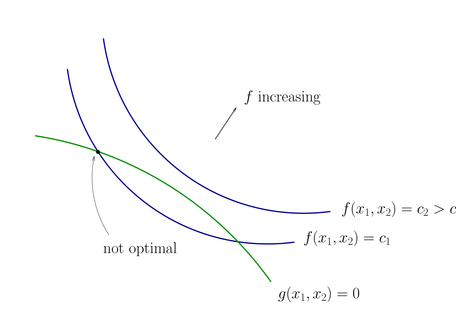
Fig. 73 Contours for \(f\) and \(g\)#
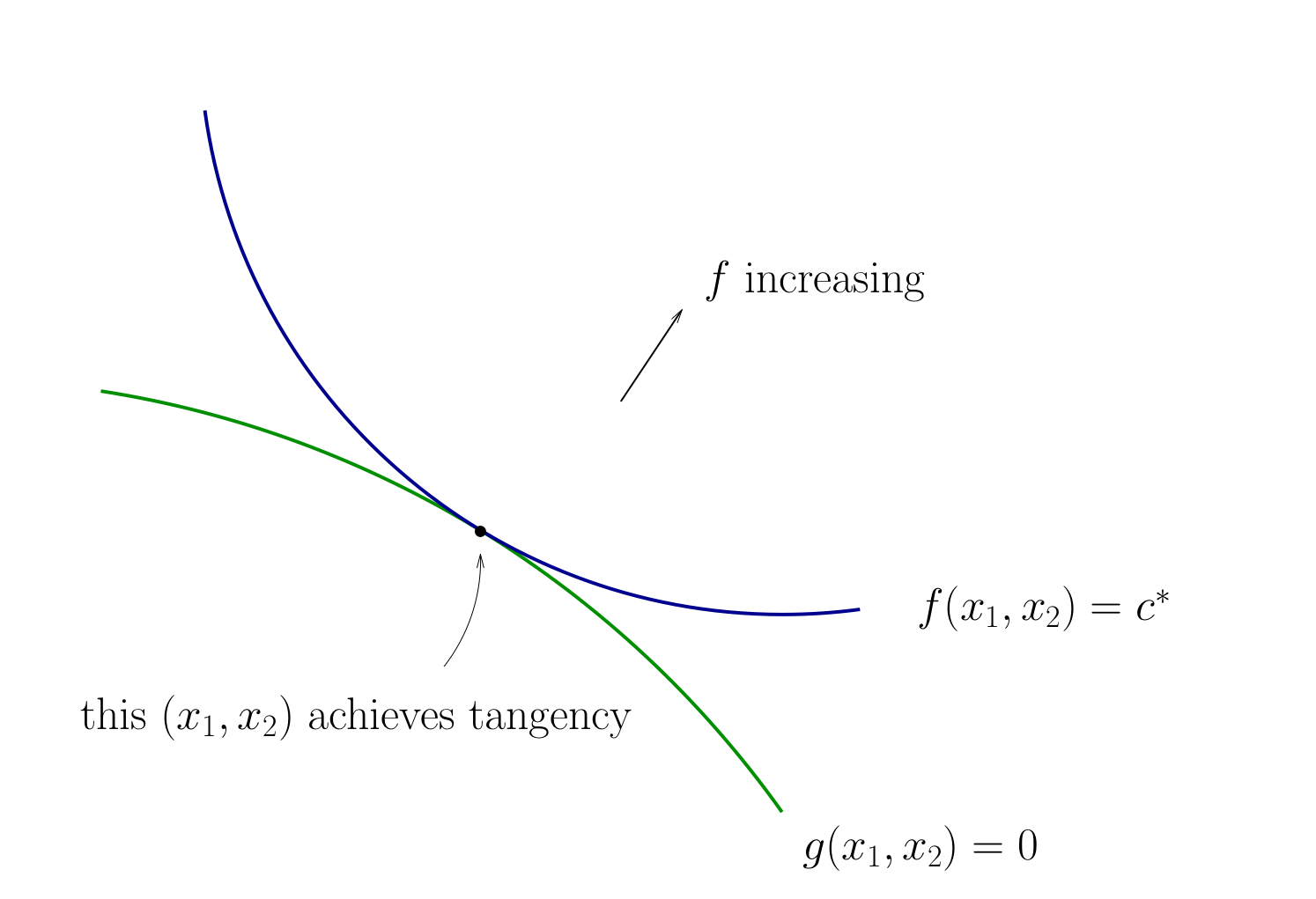
Fig. 74 Tangency necessary for optimality#
How do we locate an optimal \((x_1, x_2)\) pair?
Diversion: derivative of an implicit function
To continue with the tangency approach we need to know how to differentiate an implicit function \(x_2(x_1)\) which is given by a contour line of the utility function \(f(x_1, x_2)=c\)
Let’s approach this task in the following way
utility function is given by \(f \colon \mathbb{R}^2 \to \mathbb{R}\)
the contour line is given by \(f(x_1,x_2) = c\) which defines an implicit function \(x_1(x_2)\)
let map \(g \colon \mathbb{R} \to \mathbb{R}^2\) given by \(g(x_2) = \big[x_1(x_2),x_2\big]\)
The total derivative matrix of \(f \circ g\) can be derived using the chain rule
Differentiating the equation \(f(x_1,x_2) = c\) on both sides with respect to \(x_2\) gives \(D(f \circ g)(x) = 0\), thus leading to the final expression for the derivative of the implicit function
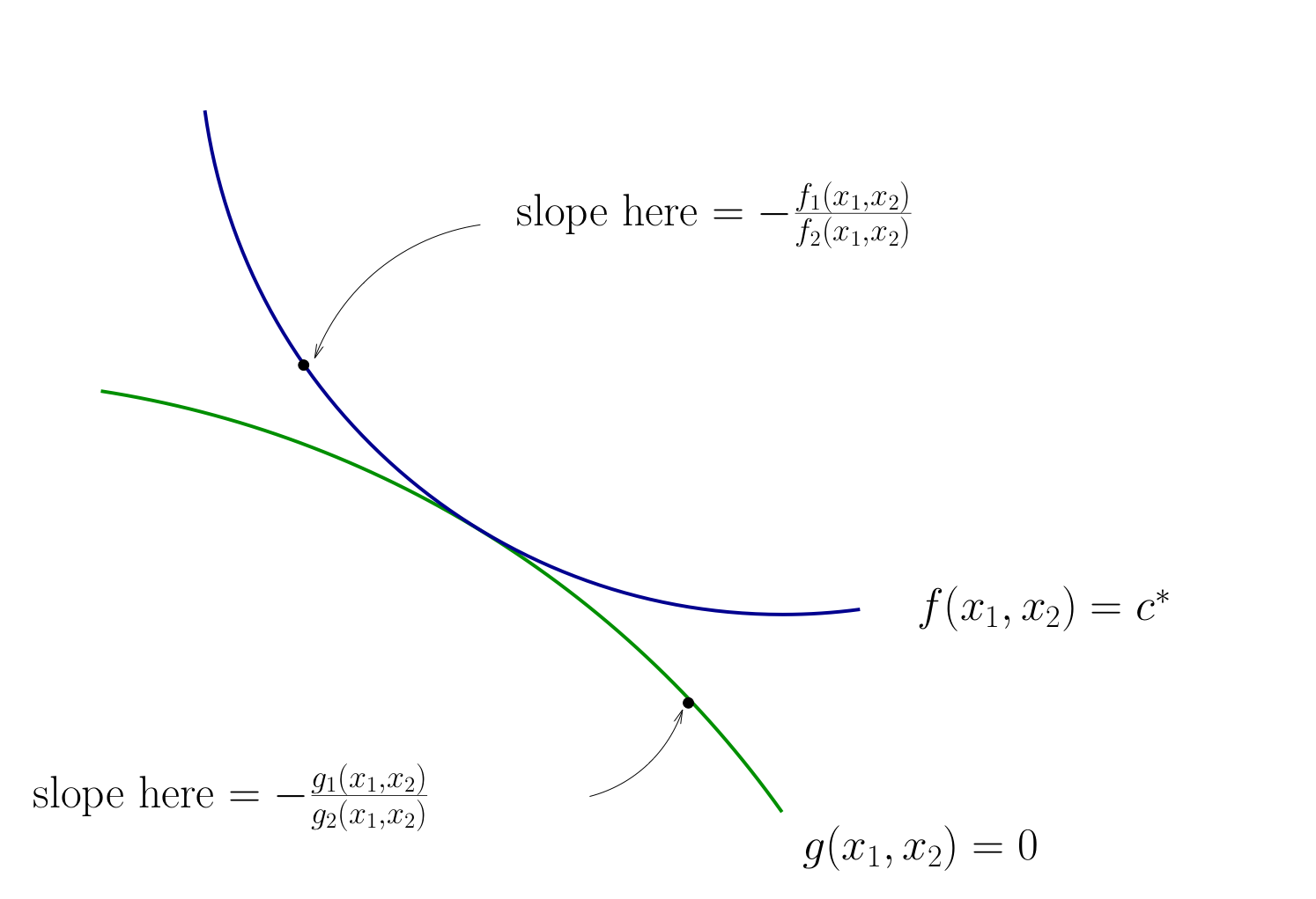
Fig. 75 Slope of contour lines#
Let’s choose \((x_1, x_2)\) to equalize the slopes
That is, choose \((x_1, x_2)\) to solve
Equivalent:
Also need to respect \(g(x_1, x_2) = 0\)
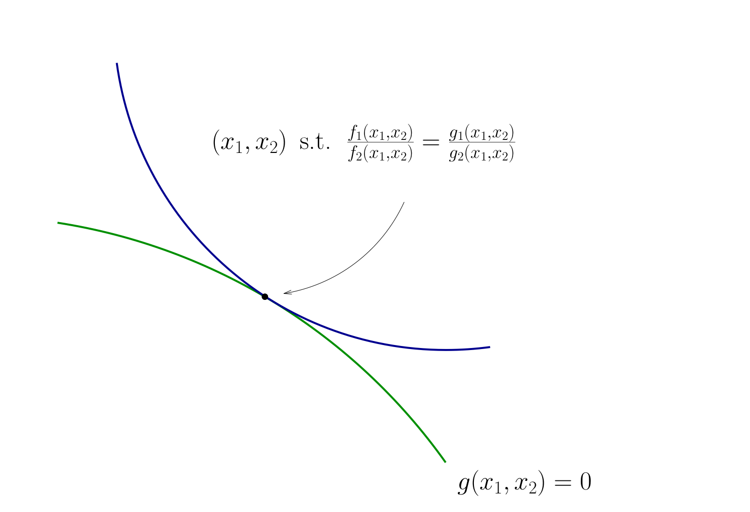
Fig. 76 Condition for tangency#
Tangency condition algorithm#
In summary, when \(f\) and \(g\) are both differentiable functions, to find candidates for optima in
(Impose slope tangency) Set
(Impose constraint) Set \(g(x_1, x_2) = 0\)
Solve simultaneously for \((x_1, x_2)\) pairs satisfying these conditions
Example
Consider again
Then
Solving simultaneously with \(p_1 x_1 + p_2 x_2 = m\) gives
Same as before…
This approach can be applied to maximization as well as minimization problems
The method of Lagrange multipliers#
Most general method for equality constrained optimization
Lagrange theorem
Let \(f \colon \mathbb{R}^N \to \mathbb{R}\) and \(g \colon \mathbb{R}^N \to \mathbb{R}^K\) be continuously differentiable functions.
Let \(D = \{ x \colon g_i(x) = 0, i=1,\dots,K \} \subset \mathbb{R}^N\)
Suppose that
\(x^\star \in D\) is a local extremum of \(f\) on \(D\), and
the gradients of the constraint functions \(g_i\) are linearly independent at \(x^\star\) (equivalently, the rank of the Jacobian matrix \(Dg(x^\star)\) is equal to \(K\))
Then there exists a vector \(\lambda^\star \in \mathbb{R}^K\) such that
Proof
See Sundaram 5.6, 5.7
Note
\(\lambda^\star\) is called the vector of Lagrange multipliers
The assumption that the gradients of the constraint functions \(g_i\) are linearly independent at \(x^\star\) is called the constraint qualification assumption
Lagrange theorem provides necessary first order conditions for both maximum and minimum problems
Definition
The function \(\mathcal{L} \colon \mathbb{R}^{N+K} \to \mathbb{R}\) defined as
is called a Lagrangian (function)
Different sources define the Lagrangian with minus or plus in front of the second term: mathematically the two definitions are equivalent, but the choice of the sign affects the interpretation of the Lagrange multipliers
I like to have a minus in the Lagrangian for consistency with the inequality constrained case where the sign is important
We come back to this in the next lecture
Fact
First order conditions for the Lagrangian coincide with the conditions in the Lagrange theorem, and together with the constraint qualification assumption they provide necessary first order conditions for the constrained optimization problem.
Example
Form the Lagrangian
FOC
From the first two equations we have \(x_1 = \frac{\alpha}{\lambda p_1}\) and \(x_2 = \frac{\beta}{\lambda p_2}\), and then from the third one \(\frac{\alpha}{\lambda} + \frac{\beta}{\lambda} = m\). This gives \(\lambda = \frac{\alpha + \beta}{m}\), leading to the same result
Lagrangian as tangency condition#
Set
and solve the system of
We have
Hence \(\frac{\partial \mathcal{L}}{\partial x_1} = \frac{\partial \mathcal{L}}{\partial x_2} = 0\) gives
Finally
Hence the method leads us to the same conditions as the tangency condition method!
Second order conditions#
similar to the unconstrained case, but applied to the Lagrangian
have to do with local optima only
similarly, provide sufficient conditions in the strict case, but only necessary conditions in the weak case
Using the rules of the differentiation from multivariate calculus we can express the gradient and the Hessian of the Lagrangian w.r.t. \(x\) as
\(\odot\) denotes multiplication of the vector \(\lambda\) and the Hessian \((K,N,N)\) tensor \(Hg(x)\) along the first dimension
Fact (necessary SOC)
Let \(f \colon \mathbb{R}^N \to \mathbb{R}\) and \(g \colon \mathbb{R}^N \to \mathbb{R}^K\) be twice continuously differentiable functions (\(C^2\)) and let \(D = \{ x \colon g_i(x) = 0, i=1,\dots,K \} \subset \mathbb{R}^N\)
Suppose \(x^\star \in D\) is the local constrained optimizer of \(f\) on \(D\) and that the constraint qualification assumption holds at \(x^\star\) and some \(\lambda^\star \in \mathbb{R}^K\)
Then:
If \(f\) has a local maximum on \(D\) at \(x^\star\), then \(H_x \mathcal{L}(\lambda,x)\) defined above is negative semi-definite on a linear constraint set \(\{v: Dg(x^\star) v = 0\}\), that is
If \(f\) has a local minimum on \(D\) at \(x^\star\), then \(H_x \mathcal{L}(\lambda,x)\) defined above is positive semi-definite on a linear constraint set \(\{v: Dg(x^\star) v = 0\}\), that is
Fact (sufficient SOC)
Let \(f \colon \mathbb{R}^N \to \mathbb{R}\) and \(g \colon \mathbb{R}^N \to \mathbb{R}^K\) be twice continuously differentiable functions (\(C^2\)) and let \(D = \{ x \colon g_i(x) = 0, i=1,\dots,K \} \subset \mathbb{R}^N\)
Suppose there exists \(x^\star \in D\) such that \(\mathrm{rank}(Dg(x^\star)) = K\) and \(Df(x^\star) - \lambda^\star \cdot Dg(x^\star) = 0\) for some \(\lambda^\star \in \mathbb{R}^K\) (the constraint qualification assumption holds at \(x^\star\) which satisfies the FOC)
Then:
If \(H_x \mathcal{L}(\lambda,x)\) defined above is negative definite on a linear constraint set \(\{v: Dg(x^\star) v = 0\}\), that is
then \(x^\star\) is the local constrained maximum of \(f\) on \(D\)
If \(H_x \mathcal{L}(\lambda,x)\) defined above is positive definite on a linear constraint set \(\{v: Dg(x^\star) v = 0\}\), that is
then \(x^\star\) is the local constrained minimum of \(f\) on \(D\)
Thus, the structure of both the necessary and the sufficient conditions is very similar to the unconstrained case.
The important difference is that the definiteness of the Hessian is checked on the linear constraint set \(\{v: Dg(x^\star) v = 0\}\) rather than on the whole \(\mathbb{R}^N\).
The linear constraint set represents the tangent hyperplane to the constraint set at \(x^\star\).
But how do we check for definiteness on a linear constraint set?
Bordered Hessian#
Let’s start with an example where we just apply the unconstrained second order conditions to the Lagrangian function
Example
The Lagrangian is
The first order conditions are then
Adding the first and second equation, we get \(2\lambda(x^2+y^2) = 4\), and therefore combining with the third, \(\lambda = 2\). From this, \(x^2 = 1/4\), \(x = 1/2\), and \(y^2 = 3/4\), \(y = \sqrt{3}/2\) (taking only the positive solutions as required).
The Hessian of the Lagrangian function is traditionally written with Lagrange multipliers as first variables, so we have
Evaluated at the stationary point \((1/2,\sqrt{3}/2)\) and \(\lambda=2\)
The leading principle minors are \(0\), \(-1\) and \(32\) which does not fit any of the five patterns of the Silvester criterion.
THIS IS WRONG
The problem can be solved by substitution \(y = \sqrt{1-x^2}\) and it’s not too hard to show that the resulting one-dimensional objective is concave.
We need new theory!
Note that the upper left corner in the Hessian of the Lagrangian is always zero
Definition
The Hessian of the Lagrangian with respect to \((\lambda, x)\) is caleld a bordered Hessian, and is given by
Note that the bordered Hessian \(H \mathcal{L}(\lambda,x)\) is different from the Hessian of the Lagrangian w.r.t. \(x\) denoted above as \(H_x \mathcal{L}(\lambda,x)\)
\(H \mathcal{L}(\lambda,x)\) is \((N+K \times N+K)\) matrix
\(H_x \mathcal{L}(\lambda,x)\) is \((N \times N)\) matrix
The bordered Hessian can be derived by differentiating the gradient
with respect ot \((\lambda,x)\), using the standard approach from multivariate calculus
the subscripts in the definition above denote the shape of the blocks in the bordered Hessian
by convention the Lagrange multipliers are placed before the other variables.
however, some textbooks place the “border”, i.e. Jacobians of the constrained in upper left corner and the Hessian w.r.t. \(x\) of the objective in the lower right corner, with corresponding changes in the propositions below
the sign for the second term in the Lagrangian also appears and may differ between different texts
Diversion: definiteness of quadratic form subject to linear constraint#
Let us review the theory using simpler case of quadratic forms
Definition
Let \(x \in \mathbb{R}^N\), \(A\) is \((N \times N)\) symmetric matrix and \(B\) is \((K \times N)\) matrix.
Quadratic form \(Q(x)\) is called positive definite subject to a linear constraint \(Bx=0\) if
Quadratic form \(Q(x)\) is called negative definite subject to a linear constraint \(Bx=0\) if
Positive and negative semi-definiteness subject to a linear constraint is obtained by replacing strict inequalities with non-strict ones.
recall that \(Bx=0\) is equivalent to saying that \(x\) is in the null space (kernel) of \(B\)
we assume that \(N>K\), so that null space of \(B\) has non-zero dimension \(N-K\)
we also assume that \(\mathrm{rank}(B)=K\), so that no two rows of \(B\) are linearly dependent, that is each constraint is important
Without loss of generality (due to reordering of the variables) we can decompose \((K \times M)\) matrix \(B\) as
\(B_2\) is then a \((K \times N-K)\) matrix representing the basis for the null space of \(B\).
Then the following derivation allows to express the null space of \(B\) through \((x_{K+1},\dots,x_N)\) as parameters
The newly denoted matrix \(J\) is \((K \times N-K)\). We can write the full vector \(x: Bx=0\) in terms of the truncated vector \(\hat{x}=(x_{K+1},\dots,x_{N})\) which plays the role of parameters. Using matrix \(J\) and the \((N-K \times N-K)\) identity matrix \(I_{N-K}\) we have
With this, the original quadratic form \(x^TAx\) subject to the linear constraint can be rewritten as
We have a new quadratic form which is a map \(\mathbb{R}^{N-K} \to \mathbb{R}\) and is defined by the \((N-K \times N-K)\) symmetric matrix
The original quadratic form \(x^T A x\) evaluated at \(x\) which satisfies \(Bx=0\) returns the same value as the new quadratic form \(\hat{x}^T E \hat{x}\) evaluated at the corresponding \(\hat{x}=(x_{K+1},\dots,x_N)\). Therefore we can study the definiteness of quadratic form \(E\) instead of definiteness of the original quadratic form subject to the linear constraint!
Direct computation of \(E\) requires the inversion of \(B_1\) which is inconvenient. To study the definiteness of \(E\) conveniently, consider a \((N+K \times N+K)\) bordered matrix
where \(A_{ij}\) are appropriately sized blocks of matrix \(A\). Namely \(A_{11}\) is \((K \times K)\), \(A_{22}\) is \((N-K \times N-K)\), and \(A_{12}\) and \(A_{21}\) are \((K \times N-K)\) and \((N-K \times K)\) respectively.
Bordered matrixes are useful as most matrix arithmetic operations can be performed on bordered matrices as if the blocks were individual scalar elements. For example, with an additional (change-of-basis) block matrix
we have
Note that \(B_1 J + B_2 = B_1 (-B_1^{-1}B_2) + B_2 = 0\). Further, let \(C=A_{11}J+A_{12}\), and then \(C^{T}=J^TA_{11}^T+A_{12}^T=J^TA_{11}+A_{21}\) since \(A\) is symmetric
To verify that the lower right block is just \(E\), apply the decomposition of \(A\) into blocks to the definition of \(E\) above:
Next, let’s compute the determinant of bordered matrix \(H\). First, note that the determinant of the diagonal change of basis matrix is 1 (the product of the elements on the diagonal):
And therefore due to the determinant of the product rule, we have
Next we will use the following formula for square block matrices, where \(W_1\) and \(W_2\) are square:
We have
The \((-1)^K\) coefficient is due to the fact that we swapped \(K\) rows (generally, swapping two rows is the same as multiplying a matrix to a permutation matrix which determinant is in this case -1). Applying the formula for block determinant and determinant of transpose matrix (twice), we have
We conclude that the sign of \(\det E\) corresponds to the sign of bordered matrix \(\det H\) directly, corrected by the number of linear constraints \(K\).
Importantly, the same derivation holds for each principle minor of \(E\)
Therefore, the definiteness of the quadratic form given by \(E\) can be checked by examining the determinants of the matrixes obtained form the bordered \(H\) by removing certain columns and rows from the last \(N-K\) columns and rows.
To examine the signs of the leading principle minors of order \(j\), the last \(j\) columns and bottom \(j\) rows have to be removed, for \(j=1,\dots,N-K\). To examine the signs of any principle minors of order \(j\), any \(j\) columns and rows (with the same index, i.e. corresponding to a diagonal element) have to be removed among the last \(N-K\) columns and rows.
Let’s compute the order-\(j\) leading principle minor of \(E\) through the elements of the bordered matrix \(H\). Denote the matrix composed on the first \(j\) columns and first \(j\) rows of \(E\) by \(E^j\):
Here all the relevant matrixes are truncated such that dimension \(N-K\) is replaced by \(j\):
\(J^j\) is \((K \times j)\) matrix formed of the first \(j\) columns of \(J\), \((K \times j)\) matrix
\(A^j_{22}\) is the first \(j\) rows and columns of the block \(A_{22}\), \((j \times j)\) matrix
\(A^j_{12}\) is the first \(j\) columns of the block \(A_{12}\), \((K \times j)\) matrix
\(A^j_{21}\) is the first \(j\) rows of the block \(A_{21}\), \((j \times K)\) matrix
\(I_j\) is \((j \times j)\) identity matrix
We have
where \(H^j\) is given by \(H\) with the last \((N-K-j)\) rows and columns removed:
where \(B^j_2\) is buit in similar manner to all other truncated matriced: these are the first \(j\) columns of the matrix \(B_2\), \((K \times j)\) matrix
In other words, the oder-\(j\) leading principle minor of \(E\) is given by the determinant of the bordered matrix \(H\) where the last \((N-K-j)\) rows and columns are dropped
Definiteness of quadratic form subject to linear constraint
In order to establish definiteness of the quadratic form \(x^TAx\), \(x \in \mathbb{R}^N\), subject to a linear constraint \(Bx=0\), we need to check signs of the \(N-K\) leading principle minors of the \((N-K \times N-K)\) matrix \(E\) which represents the equivalent lower dimension quadratic form without the constraint. The signs of these leading principle minors correspond to \((-1)^K\) times the signs of the determinant of the corresponding bordered matrix \(H\), where a number of last rows and columns are dropped, according to the following table:
Order \(j\) of leading principle minor in \(E\) |
Include first rows/columns of \(H\) |
Drop last rows/columns of \(H\) |
|---|---|---|
1 |
\(2K+1\) |
\(N-K-1\) |
2 |
\(2K+2\) |
\(N-K-2\) |
\(\vdots\) |
\(\vdots\) |
\(\vdots\) |
\(N-K-1\) |
\(N+K-1\) |
1 |
\(N-K\) |
\(N+K\) |
0 |
Clearly, this table has \(N-K\) rows, and it is \(N-K\) determinants that have to be computed.
The definiteness of the quadratic form subject to the linear constraint is then given by the pattern of signs of these determinants according to the Silvester’s criterion.
Note that computing determinants of \(H\) after dropping a number of last rows and columns is effectively computing last leading principle minors of \(H\).
If any of the leading principle minors turns out to be zero, we can move on and check the patters for the semi-definiteness.
To establishing semi-definiteness we have to do a bit more work because not only the signs of the leading principal minors, but the signs of all principle minors have to be inspected.
Semi-definiteness of quadratic form subject to linear constraint
In order to establish semi-definiteness of the quadratic form \(x^TAx\), \(x \in \mathbb{R}^N\), subject to a linear constraint \(Bx=0\), we need to check signs of the principle minors of the \((N-K \times N-K)\) matrix \(E\) which represents the equivalent lower dimension quadratic form without the constraint. The signs of these principle minors correspond to \((-1)^K\) times the signs of the determinant of the corresponding bordered matrix \(H\), where a number number of rows and columns are dropped from among the last \(N-K\) rows and columns (in all combinations), according to the following table:
Order \(j\) of principle minor in \(E\) |
Number of principle minors |
Drop among last \(N-K\) rows/columns |
|---|---|---|
1 |
\(N-K\) |
\(N-K-1\) |
2 |
\(C(N-K,2)\) |
\(N-K-2\) |
\(\vdots\) |
\(\vdots\) |
\(\vdots\) |
\(N-K-1\) |
\(N-K\) |
1 |
\(N-K\) |
1 |
0 |
The table again has \(N-K\) rows, but each row corresponds to a different number of principle minors of a given order, namely for order \(j\) there are \((N-k)\)-choose-\(j\) principle minors given by the corresponding number of combinations \(C(N-K,j)\).
The total number of principle minors to be checked is \(2^{N-K}-1\), given by the sum of binomial coefficients
The definiteness of the quadratic form subject to the linear constraint is then given by the pattern of signs of these determinants according to the Silvester’s criterion.
In what follows we will refer to computing determinants of \(H\) after dropping a number of rows and columns among the last \(N-K\) rows and columns as computing last principle minors of \(H\). The number of last principle minors will correspond to the number of lines in the table above, and not the number of determinants to be computed.
Application of the Silvester criterion for the positive definiteness and semi-definiteness is straightforward: all determinants have to be positive of non-negative, respectively.
However, let us examine the patterns of the alternating signs of the principle minors of different orders in the Silvester’s criterion for negative definiteness and semi-definiteness. The sign of the determinants corresponding to the \(j=1\) order minors has to be \((-1)(-1)^K\), and then alternate according to the following sequences:
The number of elements in these sequences that are to be checked is \(N-K\), thus the sign changes \(N-K-1\) times. Thus, the last sign is given by \((-1)(-1)^K(-1)^{N-K-1} = (-1)^N\). The highest order principle minor to check corresponds to the full determinant of the bordered matrix \(H\), and therefore it is more convenient to check the negative definiteness and semi-definiteness pattern by ensuring that:
the signs alternate for different order principle minors along the change of \(j\)
the sign of the last principle minor given by the determinant of the full bordered matrix \(H\) is \((-1)^N\)
Note that this version of the alternation rule applies for both leading principle minors and all principle minors, though in the latter case more determinants have to be checked to satisfy the sign alternation pattern.
Example
Determine the definiteness of quadratic form \(x^TAx\) subject to the linear constraint \(Bx=0\) where
Form the bordered matrix \(H\)
We have \(N=3\), \(K=1\), therefore we have to compute \(N-K=2\) determinants to check the signs of the leading principle minors of \(E\) (lower dimension unconstrained quadratic form). Note that all signs will have to be interpreted flipped, as \((-1)^K = (-1)^1 = -1\).
The sign of the first order leading principle minor of \(E\) is
The sign of the second order leading principle minor of \(E\) is
Hence, by Silvester’s criterion, the quadratic form \(x^TAx\) subject to the linear constraint \(Bx=0\) is positive definite.
Back to second order conditions#
Recall that the second order conditions of the equality constrained optimization problems are formulated in terms of the definiteness of the Hessian of the Lagrangian function with respect to \(x\), \(H_x \mathcal{L}(\lambda,x)\), subject to the linear constraint \(Dg(x^\star) x = 0\).
Therefore, all the theory on the definiteness of the quadratic form subject to the linear constraint can be applied to the bordered Hessian of the Lagrangian function \(H \mathcal{L}(\lambda,x)\).
Fact (definiteness of Hessian on linear constraint set)
For \(f \colon \mathbb{R}^N \to \mathbb{R}\) and \(g \colon \mathbb{R}^N \to \mathbb{R}^K\) twice continuously differentiable functions (\(C^2\)):
\(H_x \mathcal{L}(\lambda,x)\) is positive definite on a linear constraint set \(\{v: Dg(x^\star) v = 0\}\) \(\iff\) the last \(N-K\) leading principal minors of \(H \mathcal{L}(\lambda,x)\) are non-zero and have the same sign as \((-1)^K\).
\(H_x \mathcal{L}(\lambda,x)\) is negative definite on a linear constraint set \(\{v: Dg(x^\star) v = 0\}\) \(\iff\) the last \(N-K\) leading principal minors of \(H \mathcal{L}(\lambda,x)\) are non-zero and alternate in sign, with the sign of the full Hessian matrix equal to \((-1)^N\).
\(H_x \mathcal{L}(\lambda,x)\) is positive semi-definite on a linear constraint set \(\{v: Dg(x^\star) v = 0\}\) \(\iff\) the last \(N-K\) principal minors of \(H \mathcal{L}(\lambda,x)\) are zero or have the same sign as \((-1)^K\).
\(H_x \mathcal{L}(\lambda,x)\) is negative semi-definite on a linear constraint set \(\{v: Dg(x^\star) v = 0\}\) \(\iff\) the last \(N-K\) principal minors of \(H \mathcal{L}(\lambda,x)\) are zero or alternate in sign, with the sign of the full Hessian matrix equal to \((-1)^N\).
see above the exact definition of the last principle minors and how to count them
Similarly to the unconstrained case, when none of the listed conditions for the bordered Hessian hold, it is indefinite and the point tested by the second order conditions is not a constrained optimizer.
We can now reformulate the second order conditions for the equality constrained optimization problems in terms of signs of the last principle minors of the bordered Hessian of the Lagrangian function.
Fact (necessary SOC)
Let \(f \colon \mathbb{R}^N \to \mathbb{R}\) and \(g \colon \mathbb{R}^N \to \mathbb{R}^K\) be twice continuously differentiable functions (\(C^2\)), and let \(D = \{ x \colon g_i(x) = 0, i=1,\dots,K \} \subset \mathbb{R}^N\)
Suppose \(x^\star \in D\) is the local constrained optimizer of \(f\) on \(D\) and that the constraint qualification assumption holds at \(x^\star\) and some \(\lambda^\star \in \mathbb{R}^K\)
Then:
If \(f\) has a local maximum on \(D\) at \(x^\star\), then the last \(N-K\) principal minors of bordered Hessian \(H \mathcal{L}(\lambda,x)\) are zero or alternate in sign, with the sign of the determinant of the full Hessian matrix equal to \((-1)^N\)
If \(f\) has a local minimum on \(D\) at \(x^\star\), then the last \(N-K\) principal minors of bordered Hessian \(H \mathcal{L}(\lambda,x)\) are zero or have the same sign as \((-1)^K\)
see above the exact definition of the last principle minors and how to count them
Fact (sufficient SOC)
Let \(f \colon \mathbb{R}^N \to \mathbb{R}\) and \(g \colon \mathbb{R}^N \to \mathbb{R}^K\) be twice continuously differentiable functions (\(C^2\)) and let \(D = \{ x \colon g_i(x) = 0, i=1,\dots,K \} \subset \mathbb{R}^N\)
Suppose there exists \(x^\star \in D\) such that \(\mathrm{rank}(Dg(x^\star)) = K\) and \(Df(x^\star) - \lambda^\star \cdot Dg(x^\star) = 0\) for some \(\lambda^\star \in \mathbb{R}^K\) (i.e. the constraint qualification assumption holds at \((x^\star,\lambda^\star)\) which satisfies the FOC)
Then:
If the last \(N-K\) leading principal minors of the bordered Hessian \(H \mathcal{L}(\lambda,x)\) are non-zero and alternate in sign, with the sign of the determinant of the full Hessian matrix equal to \((-1)^N\), then \(x^\star\) is the local constrained maximum of \(f\) on \(D\)
If the last \(N-K\) leading principal minors of the bordered Hessian \(H \mathcal{L}(\lambda,x)\) are non-zero and have the same sign as \((-1)^K\), then \(x^\star\) is the local constrained minimum of \(f\) on \(D\)
Example
Let’s check the second order conditions for the consumer choice problem.
Solving FOC we have as before
To check the second order conditions compute the Hessian at \(x^\star\)
Because \(N=2\) and \(K=1\) we need to check \(N-K=1\) last lead principle minor, which is the determinant of the whole \(H\mathcal{L}(\lambda^\star,x^\star)\). Using the triangle rule for computing determinants of the \(3 \times 3\) matrix, we have
We have that the determinant of the bordered Hessian has the same sign as \((-1)^N=(-1)^2\), and the condition for sign alternation is (trivially) satisfied for \(N-K = 1\) last leading principal minors.
Hence, \(H_x \mathcal{L}(\lambda,x)\) is negative definite, implying that \(x^\star\) is the local constrained maximum of \(f\) on \(D\) by the sufficient second order condition.
Lagrangian method: algorithm#
Write down the Lagrangian function \(\mathcal{L}(x,\lambda)\)
Find all stationary points of \(\mathcal{L}(x,\lambda)\) with respect to \(x\) and \(\lambda\), i.e. solve the system of first order equations
Derive the bordered Hessian \(H \mathcal{L}(x,\lambda)\) and compute its value at the stationary points
Using second order conditions, check if the stationary points are local optima
To find the global optima, compare the function values at all identified local optima
note that using convexity/concavity of the objective function is not as straightforward as in the unconstrained case, requires additional assumptions on the convexity of the constrained set
When does Lagrange method fail?#
Example
Proceed according to the Lagrange recipe
The FOC system of equations
does not have solutions! From second equation \(\lambda \ne 0\), then from the first equation \(x=0\), and so \(y=0\) from the thrid, but then the second equation is not satisfied.
However, we can deduce that \((x^\star,y^\star)=(0,0)\) is a maximizer in the following way. For all points \((x,y)\) which satisfy the constraint \(y^3 \ge 0\) because \(x^2 \ge 0\), and thus the maximum attainable value is \(f(x,y)=0\) which it takes at \((0,0)\).
Why does Lagrange method fail?
The Lagrange method fails because the constraint qualification assumption is not satisfied at \((0,0)\), i.e. the rank of Jacobian matrix of the constraints (one by two in this case) is zero which is less than the number of constraints \(K\).
Lagrange method may not work when:
Constraints qualification assumption is not satisfied at the stationary point
FOC system of equations does not have solutions (thus no local optima)
Saddle points – second order conditions can help
Local optimizer is not a global one – no way to check without studying analytic properties of each problem
Conclusion: great tool, but blind application may lead to wrong results!
References and reading#
References
Simon & Blume: 16.2, whole of chapter 18, 19.3
Sundaram: chapters 5 and 6
Further reading and self-learning
Quadratic forms subject to linear constraints, Department of Mathematics, Northwestern University: details on definiteness subject to constraint
Second derivative test for constrained extrema, Department of Mathematics, Northwestern University: a more detailed treatment of bordered determinants