📖 Determinants, eigenpairs and diagonalization

📖 Determinants, eigenpairs and diagonalization#

⏱ | words

Determinants#

Determinant is a fundamental characteristic of any matrix $A$ and a linear operator given by a matrix $A$

Note

Determinants are only defined for square matrices, so in this section we only consider square matrices.

we use some sort of recursive definition

Definition

For a square $2 \times 2$ matrix the determinant is given by

\[\begin{split} % \det \left( \begin{array}{cc} a & b \\ c & d \\ \end{array} \right) = ad - bc % \end{split}\]

Notation for the determinant is either $\det(A)$ or sometimes $|A|$

Example

\[\begin{split} % \det \left( \begin{array}{cc} 2 & 0 \\ 7 & -1 \\ \end{array} \right) = (2 \times -1) - (7 \times 0) = -2 % \end{split}\]

We build the definition of the determinants of larger matrices from $2 \times 2$ case. Think of the next definitions as a ‘induction step’

Definition

Consider an $n \times n$ matrix $A$. Denote $A_{ij}$ a $(n-1) \times (n-1)$ submatrix of $A$, obtained by deleting the $i$-th row and $j$-th column of $A$. Then

the $(i,j)$-th minor of $A$ denoted $M_{ij}$ is

\[ M_{ij} = \det(A_{ij}) \]

the $(i,j)$-th cofactor of $A$ denoted $C_{ij}$

\[ C_{ij} = (-1)^{i+j} M_{ij} = (-1)^{i+j} \det(A_{ij}) \]

cofactors are signed minors
signs alternate in checkerboard pattern

\[\begin{split} \left[\; \begin{array}{cccccc} + & - & + & - & + & \dots \\ - & + & - & + & - & \dots \\ + & - & + & - & + & \dots \\ - & + & - & + & - & \dots \\ + & - & + & - & + & \dots \\ \vdots & \vdots & \vdots & \vdots & \vdots & \ddots \end{array} \;\right] \end{split}\]

for even $i+j$ minors and cofactors are equal

Definition

The determinant of an $n \times n$ matrix $A$ with elements $\{a_{ij}\}$ is given by

\[ \det(A) = \sum_{i=1}^n a_{ij} C_{ij} = \sum_{j=1}^n a_{ij} C_{ij} \]

for any choice of $i$ or $j$.

given that the cofactors are lower dimension determinants, we can use the same formula to compute determinants of matrices of all sizes

Example

Expanding along the first column:

\[\begin{split} \begin{array}{l} \left| \begin{array}{ccc} a_{11},& a_{12},& a_{13} \\ a_{21},& a_{22},& a_{23} \\ a_{31},& a_{32},& a_{33} \end{array} \right| = a_{11} \left| \begin{array}{ccc} a_{22},& a_{23} \\ a_{32},& a_{33} \end{array} \right| + (-1)^3 a_{21} \left| \begin{array}{ccc} a_{12},& a_{13} \\ a_{32},& a_{33} \end{array} \right| + a_{31} \left| \begin{array}{ccc} a_{12},& a_{13} \\ a_{22},& a_{23} \end{array} \right| = \\ = a_{11} (a_{22}a_{33} - a_{23}a_{32}) - a_{21} (a_{12}a_{33}-a_{13}a_{32}) + a_{31} (a_{12}a_{23}-a_{13}a_{22}) = \\ = a_{11} a_{22}a_{33} + a_{21}a_{13}a_{32} + a_{31}a_{12}a_{23} - a_{11}a_{23}a_{32} - a_{21}a_{12}a_{33} - a_{31}a_{13}a_{22} \end{array} \end{split}\]

Expanding along the top row:

\[\begin{split} \begin{array}{l} \left| \begin{array}{ccc} a_{11},& a_{12},& a_{13} \\ a_{21},& a_{22},& a_{23} \\ a_{31},& a_{32},& a_{33} \end{array} \right| = a_{11} \left| \begin{array}{ccc} a_{22},& a_{23} \\ a_{32},& a_{33} \end{array} \right| + (-1)^3 a_{12} \left| \begin{array}{ccc} a_{21},& a_{23} \\ a_{31},& a_{33} \end{array} \right| + a_{13} \left| \begin{array}{ccc} a_{21},& a_{22} \\ a_{31},& a_{32} \end{array} \right| = \\ = a_{11} (a_{22}a_{33} - a_{23}a_{32}) - a_{12} (a_{21}a_{33}-a_{23}a_{31}) + a_{13} (a_{21}a_{32}-a_{22}a_{31}) = \\ = a_{11} a_{22}a_{33} + a_{12}a_{23}a_{31} + a_{13}a_{21}a_{32} - a_{11}a_{23}a_{32} - a_{12}a_{21}a_{33} - a_{13}a_{22}a_{31} \end{array} \end{split}\]

We got exactly same result!

Fact

Determinant of $3 \times 3$ matrix can be computed by the triangles rule:

\[\begin{split} \mathrm{det} \left( \begin{array}{ccc} a_{11},& a_{12},& a_{13} \\ a_{21},& a_{22},& a_{23} \\ a_{31},& a_{32},& a_{33} \end{array} \right) = \begin{array}{l} + a_{11}a_{22}a_{33} \\ + a_{12}a_{23}a_{31} \\ + a_{13}a_{21}a_{32} \\ - a_{13}a_{22}a_{31} \\ - a_{12}a_{21}a_{33} \\ - a_{11}a_{23}a_{32} \end{array} \end{split}\]

Examples for quick computation

\[\begin{split} \mathrm{det} \left( \begin{array}{cc} 5,& 1 \\ 0,& 1 \end{array} \right) \quad \quad \mathrm{det} \left( \begin{array}{cc} 2,& 1 \\ 1,& 2 \end{array} \right) \end{split}\]

\[\begin{split} \mathrm{det} \left( \begin{array}{ccc} 1,& 5,& 8 \\ 0,& 2,& 1 \\ 0,& -1,& 2 \end{array} \right) \quad \quad \mathrm{det} \left( \begin{array}{ccc} 1,& 0,& 3 \\ 1,& 1,& 0 \\ 0,& 0,& 8 \end{array} \right) \end{split}\]

\[\begin{split} \mathrm{det} \left( \begin{array}{cccc} 1,& 5,& 8,& 17 \\ 0,& -2,& 13,& 0 \\ 0,& 0,& 1,& 2 \\ 0,& 0,& 0,& 2 \end{array} \right) \quad \quad \mathrm{det} \left( \begin{array}{ccc} 2,& 1,& 0,& 0 \\ 1,& 2,& 0,& 0 \\ 0,& 0,& 2,& 0 \\ 0,& 0,& 0,& 2 \end{array} \right) \end{split}\]

Properties of determinants#

Important facts concerning the determinants

Fact

If $I$ is the $N \times N$ identity, $A$ and $B$ are $N \times N$ matrices and $\alpha \in \mathbb{R}$, then

$\det(I) = 1$
$\det(A) = \det(A^T)$
$\det(AB) = \det(A) \det(B)$
$\det(\alpha A) = \alpha^N \det(A)$
$\det(A) = 0$ if and only if columns of $A$ are linearly dependent
$A$ is nonsingular if and only if $\det(A) \ne 0$
$\det(A^{-1}) = \frac{1}{\det(A)}$

Example

Compute the determinant of the $(n \times n)$ matrix

\[\begin{split} \det \left( \begin{array}{cccc} K,& 0,& \dots& 0 \\ 0,& K,& \dots& 0 \\ \vdots& \vdots& \ddots& \vdots \\ 0,& 0,& \dots& K \end{array} \right) = K^n \det(I) = K^n \end{split}\]

\[\begin{split} \det \left( \begin{array}{ccccc} 1,& 1,& 1,& \dots& 1 \\ 1,& 2,& 2,& \dots& 2 \\ 1,& 2,& 3,& \dots& 3 \\ \vdots& \vdots& \vdots& \ddots& \vdots \\ 1,& 2,& 3,& \dots& n \end{array} \right) = \det \left[ \left( \begin{array}{cccc} 1,& 0,& \dots& 0 \\ 1,& 1,& \dots& 0 \\ \vdots& \vdots& \ddots& \vdots \\ 1,& 1,& \dots& 1 \end{array} \right) \left( \begin{array}{cccc} 1,& 1,& \dots& 1 \\ 0,& 1,& \dots& 1 \\ \vdots& \vdots& \ddots& \vdots \\ 0,& 0,& \dots& 1 \end{array} \right) \right] = 1 \end{split}\]

Fact

If some row or column of $A$ is added to another one after being multiplied by a scalar $\alpha \ne 0$, then the determinant of the resulting matrix is the same as the determinant of $A$.

Fact

Determinant operator is linear in each row or column separately:

a common factor of the elements of any row or column of $A$ can be taken outside of the determinant operator, and
determinant of the matrix which row or column is given by a sum of conformable vectors is given by a sum of determinants of matrices with this row or column replaced by the corresponding vector

\[\begin{split} \det \left( \begin{array}{ccc} a_{11},& a_{12},& a_{13} \\ \alpha a_{21},& \alpha a_{22},& \alpha a_{23} \\ a_{31},& a_{32},& a_{33} \end{array} \right) = \alpha \det \left( \begin{array}{ccc} a_{11},& a_{12},& a_{13} \\ a_{21},& a_{22},& a_{23} \\ a_{31},& a_{32},& a_{33} \end{array} \right) = \det \left( \begin{array}{ccc} a_{11},& \alpha a_{12},& a_{13} \\ a_{21},& \alpha a_{22},& a_{23} \\ a_{31},& \alpha a_{32},& a_{33} \end{array} \right) \end{split}\]

\[\begin{split} \det \left( \begin{array}{ccc} a_{11},& a_{12},& a_{13} \\ a_{21}+b_{1},& \alpha a_{22}+b_{2},& \alpha a_{23}+b_{3} \\ a_{31},& a_{32},& a_{33} \end{array} \right) = \det \left( \begin{array}{ccc} a_{11},& a_{12},& a_{13} \\ a_{21},& a_{22},& a_{23} \\ a_{31},& a_{32},& a_{33} \end{array} \right) + \det \left( \begin{array}{ccc} a_{11},& a_{12},& a_{13} \\ b_{1},& b_{2},& b_{3} \\ a_{31},& a_{32},& a_{33} \end{array} \right) \end{split}\]

very useful in practical computation of determinant exercises!
see Problem Set $\eta$

Where determinants are used#

Fundamental properties of the linear operators given by the corresponding matrix
Inversion of matrices
Solving systems of linear equations (Cramer’s rule)
Finding Eigenvalues and eigenvectors (soon)
Determining positive definiteness of matrices
etc, etc.

Eigenvalues and Eigenvectors#

Let $A$ be a square matrix

Think of $A$ as representing a mapping $x \mapsto A x$, this is a linear function (see prev lecture)

But sometimes $x$ will only be scaled:

\[ % A x = \lambda x \quad \text{for some scalar $\lambda$} % \]

Definition

If $A x = \lambda x$ holds and $x$ is nonzero, then

$x$ is called an eigenvector of $A$ and $\lambda$ is called an eigenvalue
$(x, \lambda)$ is called an eigenpair

Clearly $(x, \lambda)$ is an eigenpair of $A$ $\implies$ $(\alpha x, \lambda)$ is an eigenpair of $A$ for any nonzero $\alpha$

Example

Let

\[\begin{split} % A = \begin{pmatrix} 1 & -1 \\ 3 & 5 \end{pmatrix} % \end{split}\]

Then

\[\begin{split} % \lambda = 2 \quad \text{ and } \quad x = \begin{pmatrix} 1 \\ -1 \end{pmatrix} % \end{split}\]

form an eigenpair because $x \ne 0$ and

\[\begin{split} % A x = \begin{pmatrix} 1 & -1 \\ 3 & 5 \end{pmatrix} \begin{pmatrix} 1 \\ -1 \end{pmatrix} = \begin{pmatrix} 2 \\ -2 \end{pmatrix} = 2 \begin{pmatrix} 1 \\ -1 \end{pmatrix} = \lambda x % \end{split}\]

import numpy as np
A = [[1, 2],
     [2, 1]]
eigvals, eigvecs = np.linalg.eig(A)
for i in range(eigvals.size):
  x = eigvecs[:,i]
  lm = eigvals[i]
  print(f'Eigenpair {i}:\n{lm:.5f} --> {x}')
  print(f'Check Ax=lm*x: {np.dot(A, x)} = {lm * x}')

Eigenpair 0:
3.00000 --> [0.70710678 0.70710678]
Check Ax=lm*x: [2.12132034 2.12132034] = [2.12132034 2.12132034]
Eigenpair 1:
-1.00000 --> [-0.70710678  0.70710678]
Check Ax=lm*x: [ 0.70710678 -0.70710678] = [ 0.70710678 -0.70710678]

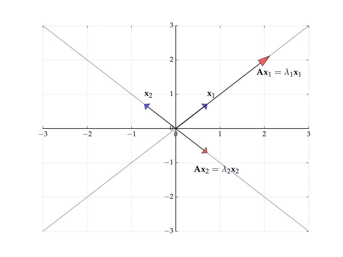
_images/eigenvecs.png — Fig. 65 The eigenvectors of $A$#

Consider the matrix

\[\begin{split} % R = \left( \begin{array}{cc} 0 & -1 \\ 1 & 0 \\ \end{array} \right) % \end{split}\]

Induces counter-clockwise rotation on any point by $90^{\circ}$

Hint

The rows of the matrix show where the classic basis vectors are translated to.

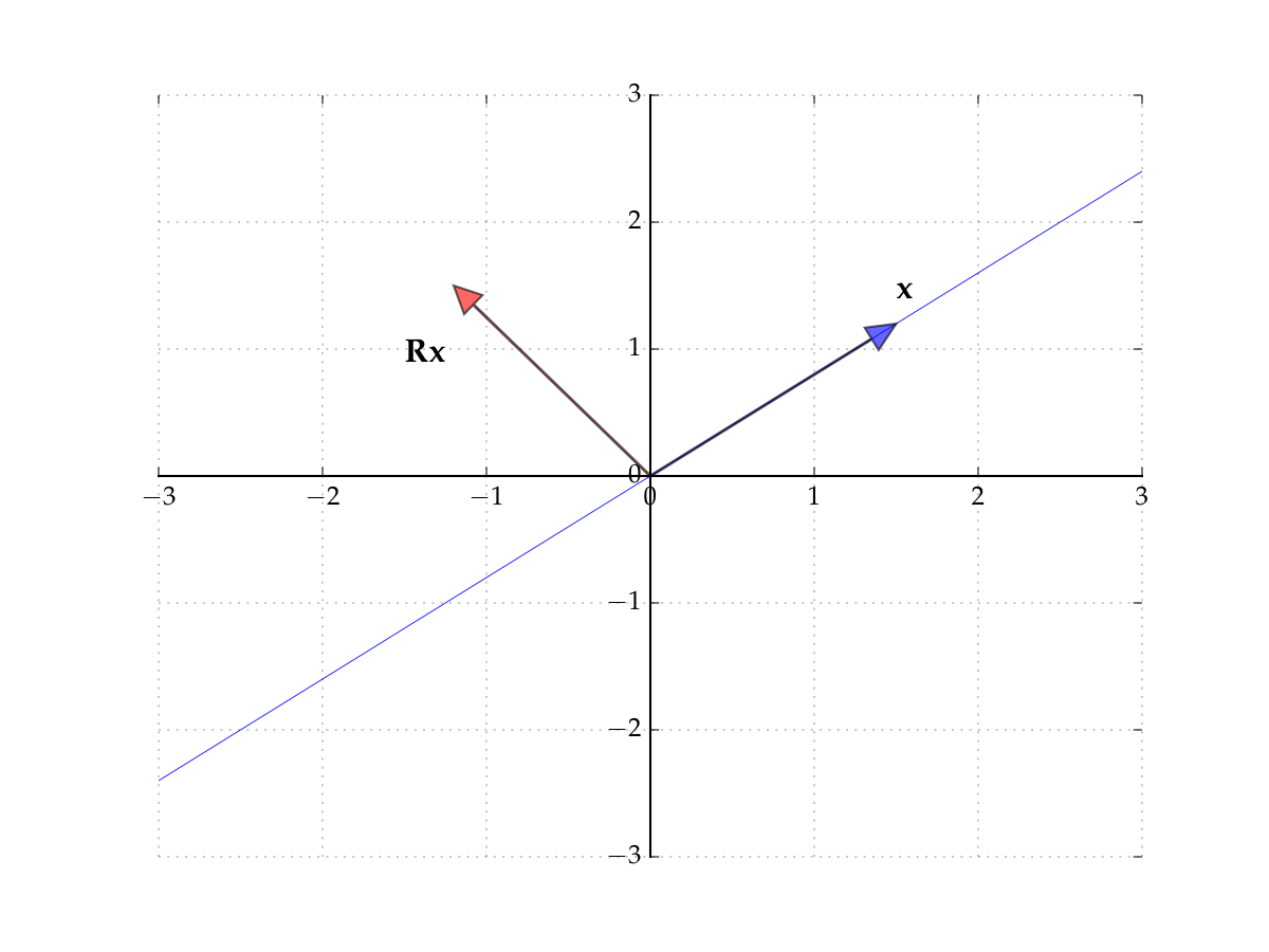
_images/rotation_1.png — Fig. 66 The matrix $R$ rotates points by $90^{\circ}$#

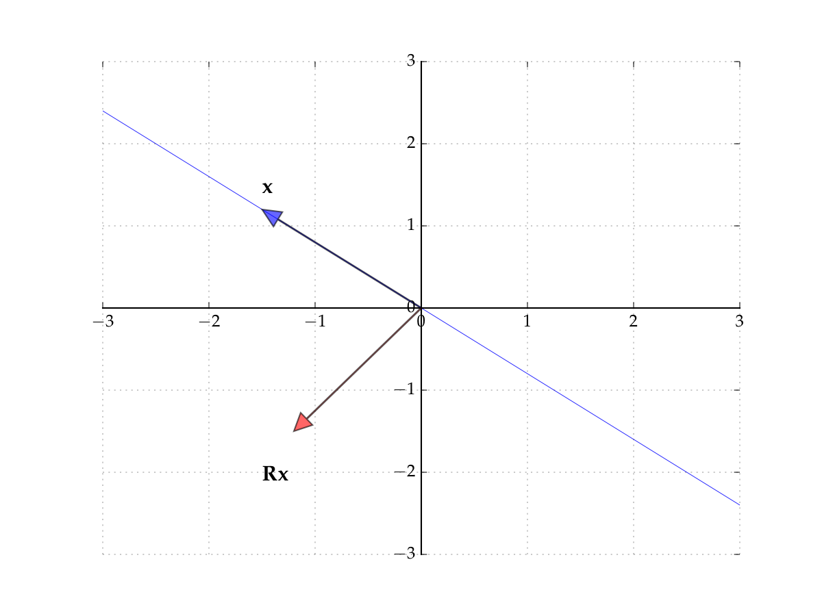
_images/rotation_2.png — Fig. 67 The matrix $R$ rotates points by $90^{\circ}$#

Hence no point $x$ is scaled

Hence there exists no pair $\lambda \in \mathbb{R}$ and $x \ne 0$ such that

\[R x = \lambda x\]

In other words, no real-valued eigenpairs exist. However, if we allow for complex values, then we can find eigenpairs even for this case

Eigenvalues and determinants#

Fact

For any square matrix $A$

\[ % \lambda \text{ is an eigenvalue of } A \; \iff \; \det(A - \lambda I) = 0 % \]

Proof

Let $A$ by $N \times N$ and let $I$ be the $N \times N$ identity

We have

\[\begin{split} % \det(A - \lambda I) = 0 \iff A - \lambda I \text{ is singular} \\ \iff \exists \, x \ne 0 \text{ such that } (A - \lambda I) x = 0 \\ \iff \exists \, x \ne 0 \text{ such that } A x = \lambda x \\ \iff \lambda \text{ is an eigenvalue of } A % \end{split}\]

Example

In the $2 \times 2$ case,

\[\begin{split} % A = \left( \begin{array}{cc} a & b \\ c & d \\ \end{array} \right) \quad \implies \quad A - \lambda I = \left( \begin{array}{cc} a - \lambda & b \\ c & d - \lambda \end{array} \right) % \end{split}\]

\[\begin{split} % \implies \det(A - \lambda I) = (a - \lambda)(d - \lambda) - bc \\ = \lambda^2 - (a + d) \lambda + (ad - bc) % \end{split}\]

Hence the eigenvalues of $A$ are given by the two roots of

\[ % \lambda^2 - (a + d) \lambda + (ad - bc) = 0 % \]

Equivalently,

\[ % \lambda^2 - \mathrm{trace}(A) \lambda + \det(A) = 0 % \]

Existence of Eigenvalues#

For an $(N \times N)$ matrix $A$ expression $\det(A - \lambda I) = 0$ is a polynomial equation of degree $N$ in $\lambda$

to see this, imagine how $\lambda$ enters into the computation of the determinant using the definition along the first row, then first row of the first minor submatrix, and so on
the highest degree of $\lambda$ is then the same as the dimension of $A$

Definition

The polynomial $\det(A - \lambda I)$ is called a characteristic polynomial of $A$.

The roots of the characteristic equation $\det(A - \lambda I) = 0$ determine all eigenvalues of $A$.

By the Fundamental theorem of algebra there are $N$ of such (complex) roots $\lambda_1, \ldots, \lambda_N$, and we can write

\[ % \det(A - \lambda I) = \prod_{n=1}^N (\lambda_n - \lambda) % \]

Each such $\lambda_i$ is an eigenvalue of $A$ because

\[ % \det(A - \lambda_i I) = \prod_{n=1}^N (\lambda_n - \lambda_i) = 0 % \]

Note: not all roots are necessarily distinct — there can be repeats

Diagonalization#

Consider a square $N \times N$ matrix $A$

\[\begin{split} % A = \left( \begin{array}{cccc} a_{11} & a_{12} & \cdots & a_{1N} \\ a_{21} & a_{22} & \cdots & a_{2N} \\ \vdots & \vdots & & \vdots \\ a_{N1} & a_{N2} & \cdots & a_{NN} \\ \end{array} \right) % \end{split}\]

Definition

The $N$ elements of the form $a_{nn}$ are called the principal diagonal

Definition

A square matrix $D$ is called diagonal if all entries off the principal diagonal are zero

\[\begin{split} % D = \left( \begin{array}{cccc} d_1 & 0 & \cdots & 0 \\ 0 & d_2 & \cdots & 0 \\ \vdots & \vdots & & \vdots \\ 0 & 0 & \cdots & d_N \\ \end{array} \right) % \end{split}\]

Often written as

\[ % D = \mathrm{diag}(d_1, \ldots, d_N) % \]

Diagonal matrixes are very nice to work with!

Example

\[\begin{split} [\mathrm{diag}(d_1, \ldots, d_N) ]^2 = \left( \begin{array}{cccc} d_1 & 0 & \cdots & 0 \\ 0 & d_2 & \cdots & 0 \\ \vdots & \vdots & & \vdots \\ 0 & 0 & \cdots & d_N \\ \end{array} \right)^2 = \left( \begin{array}{cccc} d_1^2 & 0 & \cdots & 0 \\ 0 & d_2^2 & \cdots & 0 \\ \vdots & \vdots & & \vdots \\ 0 & 0 & \cdots & d_N^2 \\ \end{array} \right) = \mathrm{diag}(d_1^2, \ldots, d_N^2) \end{split}\]

Fact

If $D = \mathrm{diag}(d_1, \ldots,d_N)$ then

$D^k = \mathrm{diag}(d^k_1, \ldots, d^k_N)$ for any $k \in \mathbb{N}$
$d_n \geq 0$ for all $n$ $\implies$ $D^{1/2}$ exists and equals

\[\mathrm{diag}(\sqrt{d_1}, \ldots, \sqrt{d_N})\]

$d_n \ne 0$ for all $n$ $\implies$ $D$ is nonsingular and

\[D^{-1} = \mathrm{diag}(d_1^{-1}, \ldots, d_N^{-1})\]

Example

Let’s find eigenvalues and eigenvectors of $D = \mathrm{diag}(d_1, \ldots,d_N)$.

The characteristic polynomial is given by

\[\begin{split} \det(D-\lambda I) = \left| \begin{array}{cccc} d_1 - \lambda & 0 & \cdots & 0 \\ 0 & d_2 - \lambda & \cdots & 0 \\ \vdots & \vdots & & \vdots \\ 0 & 0 & \cdots & d_N - \lambda \\ \end{array} \right| = \Pi_{i=1}^N (d_i - \lambda) \end{split}\]

Therefore the diagonal elements are the eigenvalues of $D$!

Change of basis#

Consider a vector $x\in \mathbb{R}^N$ which has coordinates $(x_1,x_2,\dots,x_N)$ in classis basis $(e_1,e_2,\dots,e_N)$, where $e_i = (0,\dots,0,1,0\dots,0)^T$

Coordinates of a vector is what we call the coefficients of the linear combination of the basis vectors that gives the vector

We have

\[ x = \sum_{i=1}^N x_i e_i \]

Consider a different basis in $\mathbb{R}^N$ (recall the definition) denoted $(e'_1,e'_2,\dots,e'_N)$ Here we assume that each $e'_i$ is written in the coordinates corresponding to the original basis $(e_1,e_2,\dots,e_N)$.

The coordinates of vector $x$ in basis $(e'_1,e'_2,\dots,e'_N)$ denoted $x' = (x'_1,x'_2,\dots,x'_N)$ are by definition

\[\begin{split} x = \sum_{i=1}^N x'_i e'_i = x'_1 \left( \begin{array}{c} \vdots \\ e'_1 \\ \vdots \end{array} \right) + \dots + x'_N \left( \begin{array}{c} \vdots \\ e'_N \\ \vdots \end{array} \right) = P x' \end{split}\]

Definition

The transformation matrix from the basis $(e_1,e_2,\dots,e_N)$ to $(e'_1,e'_2,\dots,e'_N)$ is given by

\[\begin{split} P = \left( \begin{array}{cccc} \vdots & \vdots & & \vdots \\ e'_1, & e'_2, & \dots & e'_N \\ \vdots & \vdots & & \vdots \end{array} \right) \end{split}\]

In other words, the same vector has coordinates $x = (x_1,x_2,\dots, x_N)$ in the original basis $(e_1,e_2,\dots,e_N)$ and $x' = (x'_1,x'_2,\dots, x'_N)$ in the new basis $(e'_1,e'_2,\dots,e'_N)$, and it holds

\[ x = P x', \quad x' = P^{-1} x \]

We now have a way to represent the same vector in different bases, i.e. change basis!

Example

\[\begin{split} \begin{array}{l} e'_1 = e_1 + e_2 \\ e'_2 = e_1 - e_2 \\ e'_3=e_3 \end{array} \implies P = \begin{pmatrix} 1 & 1 & 0 \\ 1 & -1 & 0 \\ 0 & 0 & 1 \end{pmatrix} \end{split}\]

Fact

The transformation matrix $P$ is nonsingular (invertible).

Proof

Because the transformation matrix maps a set of basis vectors to another set of basis vectors, they are linearly independent. By the properties of linear functions, $P$ is then non-singular, and $P^{-1}$ exists. $\blacksquare$

Linear functions in different bases#

Consider a linear map $A: x \mapsto Ax$ where $x \in \mathbb{R}^N$

Can we express the same linear map in a different basis?

Let $B$ be the matrix representing the same linear map in a new basis, where the transformation matrix is given by $P$.

\[ x \mapsto Ax \quad \iff \quad x' \mapsto Bx' \]

If the linear map is the same, we must have

\[ Ax = P B P^{-1}x \]

Definition

Square matrix $A$ is said to be similar to square matrix $B$ if there exist an invertible matrix $P$ such that $A = P B P^{-1}$.

Similar matrixes also happen to be very useful!

Example

Consider $A$ that is similar to a diagonal matrix $D = \mathrm{diag}(d_1,\dots,d_N)$.

To find the $A^n$ we can use the fact that

\[ A^2 = AA = P D P^{-1} P D P^{-1} = P D^2 P^{-1} \]

and therefore it’s easy to show by mathematical induction that

\[ A^k = AA = P D P^{-1} P D P^{-1} = A^k = \]

Given the properties of the diagonal matrixes, we have an easily computed expression

\[ A^k = P [\mathrm{diag}(d_1^k,\dots,d_N^k)] P^{-1} \]

Diagonalization using eigenvectors#

Definition

If $A$ is similar to a diagonal matrix, then $A$ is called diagonalizable

Fact (Diagonalizable $\longrightarrow$ Eigenpairs)

Let $A$ be diagonalizable with $A = P D P^{-1}$ and let

$D = \mathrm{diag}(\lambda_1, \ldots, \lambda_N)$
$p_n$ for $n=1,\dots,N$ be the columns of $P$

Then $(p_n, \lambda_n)$ is an eigenpair of $A$ for each $n$

Proof

From $A = P D P^{-1}$ we get $A P = P D$

Equating $n$-th column on each side gives

\[ % A p_n = \lambda_n p_n % \]

Moreover $p_n \ne 0$ because $P$ is invertible (which facts?)

Fact (Distinct eigenvalues $\longrightarrow$ diagonalizable)

If $N \times N$ matrix $A$ has $N$ distinct eigenvalues $\lambda_1, \ldots, \lambda_N$, then $A$ is diagonalizable as $A = P D P^{-1}$ where

$D = \mathrm{diag}(\lambda_1, \ldots, \lambda_N)$
each $n$-th column of $P$ is equal to the eigenvector for $\lambda_n$

Example

Let

\[\begin{split} % A = \begin{pmatrix} 1 & -1 \\ 3 & 5 \end{pmatrix} % \end{split}\]

The eigenvalues of $A$ are 2 and 4, while the eigenvectors are

\[\begin{split} % p_1 = \begin{pmatrix} 1 \\ -1 \end{pmatrix} \quad \text{and} \quad p_2 = \begin{pmatrix} 1 \\ -3 \end{pmatrix} % \end{split}\]

Hence

\[ % A = P \mathrm{diag}(2, 4) P^{-1} % \]

import numpy as np
from numpy.linalg import inv
A = np.array([[1, -1],
              [3, 5]])
eigvals, eigvecs = np.linalg.eig(A)
D = np.diag(eigvals)
P = eigvecs
print('A =',A,sep='\n')
print('D =',D,sep='\n')
print('P =',P,sep='\n')
print('P^-1 =',inv(P),sep='\n')
print('P*D*P^-1 =',P@D@inv(P),sep='\n')

A =
[[ 1 -1]
 [ 3  5]]
D =
[[2. 0.]
 [0. 4.]]
P =
[[-0.70710678  0.31622777]
 [ 0.70710678 -0.9486833 ]]
P^-1 =
[[-2.12132034 -0.70710678]
 [-1.58113883 -1.58113883]]
P*D*P^-1 =
[[ 1. -1.]
 [ 3.  5.]]

Profit!#

Fact

Given $N \times N$ matrix $A$ with distinct eigenvalues $\lambda_1, \ldots, \lambda_N$ we have

If $A = \mathrm{diag}(d_1, \ldots, d_N)$, then $\lambda_n = d_n$ for all $n$
$\det(A) = \prod_{n=1}^N \lambda_n$
If $A$ is symmetric, then $\lambda_n \in \mathbb{R}$ for all $n$ (not complex!)

Proof

The first statement can be checked directly by verifying that the classic basis vectors are eigenvectors of $A$.

The second statement follows from the properties of the determinant of a product:

\[\begin{split} \det(A) = \det(P \mathrm{diag}(\lambda_1,\dots,\lambda_N) P^{-1}) =\\= \det(P) \det(\mathrm{diag}(\lambda_1,\dots,\lambda_N)) \det(P^{-1}) =\\= det(P) \prod_{n=1}^N \lambda_n (\det(P))^{-1} = \prod_{n=1}^N \lambda_n \end{split}\]

The third statement requires complex analysis, we take for granted.

Fact

$A$ is nonsingular $\iff$ all eigenvalues are nonzero

Proof

$A$ is nonsingular $\iff$ $\det(A) \ne 0$ $\iff$ $\prod_{n=1}^N \lambda_n \ne 0$ $\iff$ all $\lambda_n \ne 0$

Fact

If $A$ is nonsingular, then eigenvalues of $A^{-1}$ are $1/\lambda_1, \ldots, 1/\lambda_N$

Proof

\[ A x = \lambda x \iff A^{-1}A x = \lambda A^{-1} x \iff x/\lambda = A^{-1} x \]

Notes from the lecture#

Hand written notes from the lecture

📖 Determinants, eigenpairs and diagonalization

Contents

📖 Determinants, eigenpairs and diagonalization#

Determinants#

Properties of determinants#

Where determinants are used#

Eigenvalues and Eigenvectors#

Eigenvalues and determinants#

Existence of Eigenvalues#

Diagonalization#

Change of basis#

Linear functions in different bases#

Diagonalization using eigenvectors#

Profit!#

Notes from the lecture#

References and reading#

References

[Simon and Blume, 1994]: chapters~9, 23 (excluding complex number)
[Sundaram, 1996]: 1.3.4-1.3.6
Further reading and self-learning
Excellent visualizations of concepts covered in this lecture, strongly recommended for further study 3Blue1Brown: Essence of linear algebra