📖 Mappings and cardinality

⏱ | words

Definition

A generic mapping \(f\) from \(A\) to \(B\) is a rule that assigns elements \(x\) of a set \(A\) to elements of a set \(B\). We write

\[f: A \to B \qquad\text{ or }\qquad f: A \ni x \mapsto f(x) \in B\]

There are four basic types of mappings:

1. A one-to-one mapping:

   • \(\forall x \in X\) there is at most one \(f(x) \in Y\); and

   • \(\forall y \in Y\) there is at most one \(x \in X\) such that \(f(x)=y\).

   • example: \(f(x) = x\)

2. A many-to-one mapping:

   • \(\forall x \in X\) there is at most one \(f(x) \in Y\); but

   • \(\exists y \in Y\) for which \(\exists x_1 \ne x_2 \in X\) such that \(f(x_1)=f(x_2)=y\).

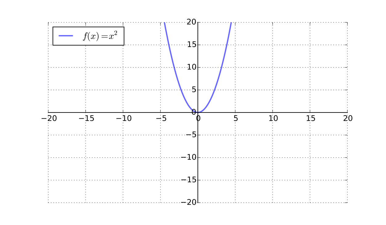
   • example: \(f(x) = x^2\)

3. A one-to-many mapping:

   • \(\exists x \in X\) for which \(\exists y_1 \ne y_2 \in f(x) \subset Y\); but

   • \(\forall y \in Y\) there is at most one \(x \in X\) such that \(f(x)=y\).

   • example: \(f(x) = \{e^x,-e^x\}\)

4. A many-to-many mapping:

   • \(\exists x \in X\) for which \(\exists y_1 \ne y_2 \in f(x) \subset Y\); but

   • \(\exists y \in Y\) for which \(\exists x_1 \ne x_2 \in X\) such that \(f(x_1)=f(x_2)=y\).

   • example: \(f(x) = \{x,x+1,x+2,\dots\}\)

Mappings of the first two types are referred to as functions. Mappings of the last two types are referred to as set-valued functions or correspondences.

Functions

Definition

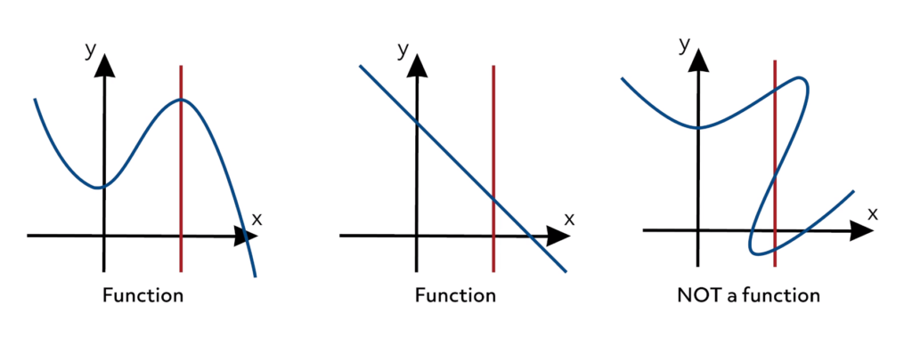
A function \(f: A \rightarrow B\) from set \(A\) to set \(B\) is a mapping that associates to each element of \(A\) a uniquely determined element of \(B\).

• typically functions map \(A\) to a (Cartesian product of) set(s) of real numbers \(\mathbb{R}^n\)

Example

• Each student gets a set of textbooks is a mapping

• Each student gets a grade between 0 and 100 is a function

Definition

\(A\) is called the domain of \(f\) and \(B\) is called the co-domain

• lower panel: functions have to map all elements in domain to a uniquely determined element in co-domain

Example

\[f(x) = \exp(-x^2)\]

is a function from \(\mathbb{R}\) to \(\mathbb{R}\). We may also write

\[\begin{split}f: \mathbb{R} \to \mathbb{R} \\ x \mapsto \exp(-x^2), \text{ or}\\ f: \mathbb{R} \ni x \mapsto \exp(-x^2) \in \mathbb{R} \end{split}\]

Definition

Functions can be:

• scalar-valued when \(n=1\), so \(f: A \to \mathbb{R}\)

• vector-valued when \(n>1\), so \(f: A \to \mathbb{R}^n\)

• univariate when \(A = \mathbb{R}\), so \(f: \mathbb{R} \to \mathbb{R}^n\)

• multivariate when \(A = \mathbb{R}^m\), so \(f: \mathbb{R}^m \to \mathbb{R}^n\)

Example: not a function

Definition

For each \(a \in A\), \(f(a) \in B\) is called the image of \(a\) under \(f\)

Definition

If \(f(a) = b\) then \(a\) is called a pre-image of \(b\) under \(f\)

Definition

The definitions of image and pre-image naturally generalize to subsets of the domain.

• For each \(X \subset A\), \(f(X) = \{f(x): x \in X\} \in B\) is called the image of \(X\) under \(f\)

• For each \(Y \subset B\), \(\{x: f(x) \in Y\} \in A\) is called the pre-image of \(Y\) under \(f\)

Each point in \(B\) can have one, many or zero pre-images

The co-domain of a function is not uniquely pinned down

Example

Consider the mapping defined by \(f(x) = \exp(-x^2)\)

All of these statements are valid:

• \(f\) a function from \(\mathbb{R}\) to \(\mathbb{R}\)

• \(f\) a function from \(\mathbb{R}\) to \((0, \infty)\)

• \(f\) a function from \(\mathbb{R}\) to \((0, 1]\)

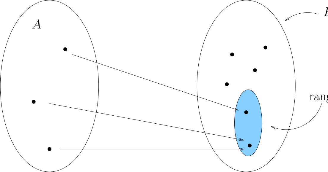
Definition

The smallest possible co-domain is called the range of \(f: A \to B\):

\[ \mathrm{rng}(f) := \{ b \in B : f(a) = b \text{ for some } a \in A \} \]

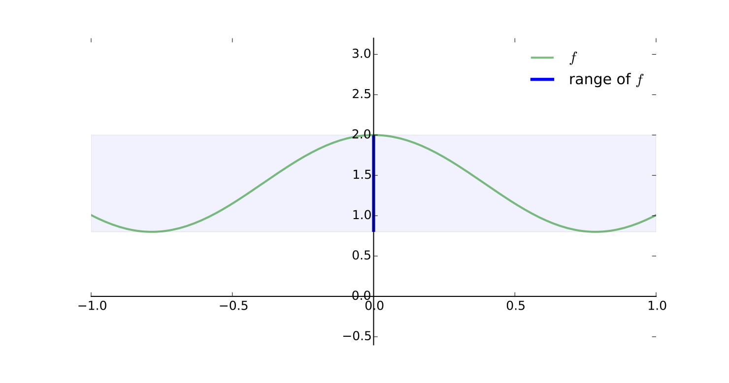
Example

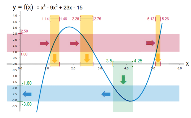
Let \(f: [-1, 1] \to \mathbb{R}\) be defined by

\[ f(x) = 0.6 \cos(4 x) + 1.4 \]

Then \(\mathrm{rng}(f) = [0.8, 2.0]\)

Example

If \( f: [0, 1] \to \mathbb{R}\) is defined by

\[ f(x) = 2x \]

then \(\mathrm{rng}(f) = [0, 2]\)

Example

If \(f: \mathbb{R} \to \mathbb{R}\) is defined by

\[ f(x) = \exp(x) \]

then \(\mathrm{rng}(f) = (0, \infty)\)

Compositions

Definition

The composition of \(f: A \to B\) and \(g: B \to C\) is the function \(g \circ f\) from \(A\) to \(C\) defined by

\[ (g \circ f)(a) = g(f(a)) \quad (a \in A) \]

Example

Let \(f: \mathbb{R} \to \mathbb{R}\) be defined by \(f(x) = x^2\) and \(g: \mathbb{R} \to \mathbb{R}\) be defined by \(g(x) = x + 1\)

Then \((g \circ f)(x) = g(f(x)) = g(x^2) = x^2 + 1\)

Note that \((f \circ g)(x) = f(g(x)) = f(x+1) = (x+1)^2 \ne (g \circ f)(x)\)

• Order of components in a composite function matters

• The domain of the outer function in a composition must contain the range of the inner function

Onto (Surjections)

Definition

A function \(f: A \to B\) is called onto (or surjection) if every element of \(B\) is the image under \(f\) of at least one point in \(A\).

Equivalently, \(\mathrm{rng}(f) = B\)

Fact

\(f: A \to B\) is onto if and only if each element of \(B\) has at least one pre-image under \(f\)

Fig. 22 Onto (surjection)

Fig. 23 Not onto!

Fig. 24 Not onto!

Example

The function \(f: \mathbb{R} \to \mathbb{R}\) defined by

\[ f(x) = ax^3 + b x^2 + cx + d \]

is onto whenever \(a \ne 0\)

To see this pick any \(y \in \mathbb{R}\)

We claim \(\exists \; x \in \mathbb{R}\) such that \(f(x) = y\)

Equivalent:

\[ \exists \; x \in \mathbb{R} \; \mathrm{s.t.} \; ax^3 + b x^2 + cx + d - y = 0 \]

Fact

Every cubic equation with \(a \ne 0\) has at least one real root

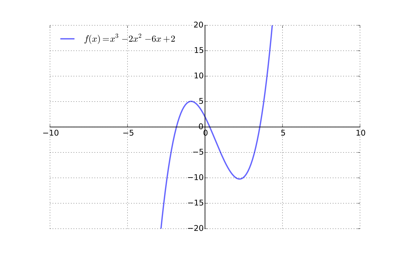
Fig. 25 Cubic functions from \(\mathbb{R}\) to \(\mathbb{R}\) are always onto

One-to-One (Injections)

Definition

A function \(f: A \to B\) is called one-to-one (or injection) if distinct elements of \(A\) are always mapped into distinct elements of \(B\).

That is, \(f\) is one-to-one if

\[ a \in A, \; a' \in A \text{ and } a \ne a' \implies f(a) \ne f(a') \]

Equivalently,

\[ f(a) = f(a') \implies a = a' \]

Fact

\(f: A \to B\) is one-to-one if and only if each element of \(B\) has at most one pre-image under \(f\)

Fig. 26 One-to-one

Fig. 27 One-to-one

Fig. 28 Not one-to-one

Bijections

Definition

A function that is

1. one-to-one (injection) and

2. onto (surjection)

is called a bijection or one-to-one correspondence

Fact

\(f: A \to B\) is a bijection if and only if each \(b \in B\) has one and only one pre-image in \(A\)

Example

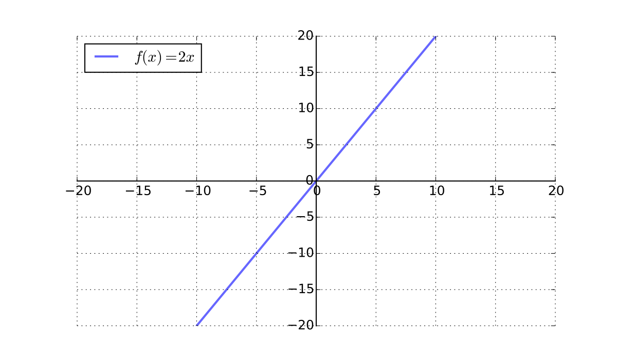
\(x \mapsto 2x\) is a bijection from \(\mathbb{R}\) to \(\mathbb{R}\)

Example

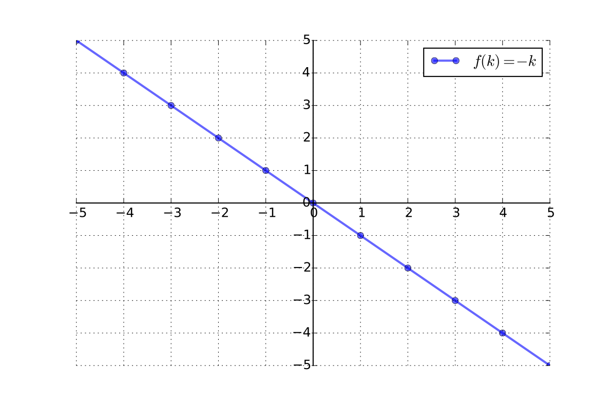
\(k \mapsto -k\) is a bijection from \(\mathbb{Z}\) to \(\mathbb{Z}\)

Example

\(x \mapsto x^2\) is not a bijection from \(\mathbb{R}\) to \(\mathbb{R} \)

Inverse functions

Fact

If \(f: A \to B\) a bijection, then there exists a unique function \(\phi: B \to A\) such that

\[ \phi(f(a)) = a, \quad \forall \; a \in A \]

That function \(\phi\) is called the inverse of \(f\) and written \(f^{-1}\)

Example

Let

• \(f: \mathbb{R} \to (0, \infty)\) be defined by \(f(x) = \exp(x) := e^x\)

• \(\phi: (0, \infty) \to \mathbb{R}\) be defined by \(\phi(x) = \log(x)\)

Then \(\phi = f^{-1}\) because, for any \(a \in \mathbb{R}\),

\[ \phi(f(a)) = \log(\exp(a)) = a \]

Fact

If \(f: A \to B\) is one-to-one, then \(f: A \to \mathrm{rng}(f)\) is a bijection

Fact

Let \(f: A \to B\) and \(g: B \to C\) be bijections

1. \(f^{-1}\) is a bijection and its inverse is \(f\)

• \(f^{-1}(f(a)) = a\) for all \(a \in A\)

• \(f(f^{-1}(b)) = b\) for all \(b \in B\)

• \(g \circ f\) is a bijection from \(A\) to \(C\) and \((g \circ f)^{-1} = f^{-1} \circ g^{-1}\)

Fig. 29 Illustration of \((g \circ f)^{-1} = f^{-1} \circ g^{-1}\)

Cardinality

If a bijection exists between sets \(A\) and \(B\) they are said to have the same cardinality, and we write \(|A| = |B|\)

Fact

If \(|A| = |B|\) and \(A\) and \(B\) are finite then \(A\) and \(B\) have the same number of elements (same cardinality).

Exercise: Convince yourself this is true

Hence “same cardinality” is analogous to “same size”

• But cardinality applies to infinite sets as well!

Fact

If \(|A| = |B|\) and \(|B| = |C|\) then \(|A| = |C|\)

Proof

• Since \(|A| = |B|\), there exists a bijection \(f: A \to B\)

• Since \(|B| = |C|\), there exists a bijection \(g: B \to C\)

Let \(h := g \circ f\)

Then \(h\) is a bijection from \(A\) to \(C\)

Hence \(|A| = |C|\)

Definition

A nonempty set \(A\) is called finite if

\[ |A| = |\{1, 2, \ldots, n\}| \quad \text{ for some } \quad n \in \mathbb{N} \]

Otherwise called infinite

Definition

Sets that either are finite, or have the same cardinality as \(\mathbb{N}\), denoted \(|A| = \aleph_0\), are called countable

Fact

A set \(X\) countable if and only if there exists a bijection \(f: X \rightarrow \mathbb{N}\).

Example

\(-\mathbb{N} := \{\ldots, -4, -3, -2, -1\}\) is countable

\[\begin{split}\begin{array}{ccc} -1 & \leftrightarrow & 1 \\ -2 & \leftrightarrow & 2 \\ -3 & \leftrightarrow & 3 \\ & \vdots & \\ -n & \leftrightarrow & n \\ & \vdots & \end{array}\end{split}\]

Formally: \(f(k) = -k\) is a bijection from \(-\mathbb{N}\) to \(\mathbb{N}\)

Example

\(E := \{2,4,6, \ldots\}\) is countable

\[\begin{split} \begin{array}{ccc} 2 & \leftrightarrow & 1 \\ 4 & \leftrightarrow & 2 \\ 6 & \leftrightarrow & 3 \\ & \vdots & \\ 2n & \leftrightarrow & n \\ & \vdots & \end{array} \end{split}\]

Formally: \(f(k) = k/2\) is a bijection from \(E\) to \(\mathbb{N}\)

Fact

Nonempty subsets of countable sets are countable

Fact

Finite unions of countable sets are countable

Proof

Sketch of proof for \(A\) and \(B\) countable \(\implies A \cup B\) countable.

Consider \(A\) and \(B\) are disjoint and infinite (the most complicated case)

By assumption, can write \(A = \{a_1, a_2, \ldots\}\) and \(B = \{b_1, b_2, \ldots\}\)

Now count it like so:

\[\begin{split} \begin{matrix} a_1 & & a_2 & & a_3 & & a_4 & \cdots\\ \downarrow & \nearrow & \downarrow & \nearrow & \downarrow & \nearrow & \downarrow & \nearrow \\ b_1 & & b_2 & & b_3 & & b_4 & \cdots \end{matrix} \end{split}\]

Example

\(\mathbb{Z} = \{\ldots, -2, -1\} \cup \{ 0 \} \cup \{1, 2, \ldots\}\) is countable

Fact

Finite Cartesian products of countable sets is countable

Proof

Sketch of proof for \(A\) and \(B\) countable \(\implies A \times B\) countable.

Consider \(A\) and \(B\) are disjoint and infinite (the most complicated case). Now count like so:

\[\begin{split} \begin{matrix} (a_{1},b_{1})&\to &(a_{1},b_{2})& & (a_{1},b_{3})&\to\cdots\\ &\swarrow& &\nearrow & & \\ (a_{2},b_{1})& &(a_{2},b_{2})& &\cdots & \\ \downarrow &\nearrow& & & & \\ (a_{3},b_{1})& &\vdots & & & \\ \vdots & & & & & \end{matrix} \end{split}\]

Example

\(\mathbb{Z} \times \mathbb{Z} = \{ (p,q) : p \in \mathbb{Z}, q \in \mathbb{Z} \}\) is countable

Fact

\(\mathbb{Q}\) is countable

Proof

By definition

\[ \mathbb{Q}:= \left\{ \, \text{all } \frac{p}{q} \text{ where } p \in \mathbb{Z} \text{ and } q \in \mathbb{N} \, \right\} \]

Consider the function \(\phi\) defined by \(\phi(p/q) = (p, q)\)

• A one-to-one function from \(\mathbb{Q}\) to \(\mathbb{Z} \times \mathbb{N}\)

• A bijection from \(\mathbb{Q}\) to \(\mathrm{rng}(\phi)\)

Since \(\mathbb{Z} \times \mathbb{N}\) is countable, so is \(\mathrm{rng}(\phi) \subset \mathbb{Z} \times \mathbb{N}\)

Hence \(\mathbb{Q}\) is also countable

Example

An example of an uncountable set is all binary sequences

\[ \{0,1\}^{\mathbb{N}} := \big\{ (b_1,b_2,\ldots) : \, b_n \in \{0,1\ \} \text{ for each } n \big\} \]

Proof

Sketch of proof: If this set were countable then it could be listed as follows:

\[\begin{split} \begin{matrix} 1 & \leftrightarrow & {\bf a_1}, \; a_2, \; a_3, \; a_4, \ldots \\ 2 & \leftrightarrow & b_1, \;{\bf b_2}, \; b_3, \; b_4, \ldots \\ 3 & \leftrightarrow & c_1, \; c_2, \;{\bf c_3}, \; c_4, \ldots \\ 4 & \leftrightarrow & d_1, \; d_2, \; d_3, \;{\bf d_4}, \ldots \\ \vdots & & \vdots \end{matrix} \end{split}\]

Such a list is never complete: Cantor’s diagonalization argument

Cardinality of \(\{0,1\}^{\mathbb{N}}\) called the power of the continuum

Other sets with the power of the continuum

• \(\mathbb{R}\)

• \((a, b)\) for any \(a < b\)

• \([a, b]\) for any \(a < b\)

• \(\mathbb{R}^N\) for any finite \(N \in \mathbb{N}\)

Continuum hypothesis

Every nonempty subset of \(\mathbb{R}\) is either countable or has the power of the continuum

• Not a homework exercise!

Example

\(\mathbb{R}\) and \((-1, 1)\) have the same cardinality because \(x \mapsto 2\arctan(x)/\pi\) is a bijection from \(\mathbb{R}\) to \((-1, 1)\)

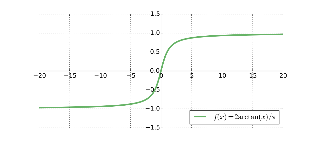
Fig. 30 Same cardinality

References and further reading

References

• [Simon and Blume, 1994]: 2.1, 2.2, 5.1

---

Mentimeter reflection