EXTRA MATERIAL
Material in this section is optional and will not be part of the course assessment.
☕️ Dynamic inventory management#
⏱ | words
This is an example of dynamic discrete choice model with numerical solution 👍
Inventory management in finite horizon#
Example
The manager of a store has to order the stock of a product from a wholesales company as the inventory is depleted by sales.
The manager can order any amount of the product at any time, but there is a fixed cost \(c\) of ordering any amount of new inventory. The manager can also store the product in the warehouse, but there is a cost \(r\) of storing one unit of the product.
The store receives a profit \(p\) for each unit of the product sold and so the manager’s goal is to maximize the net profit over the time horizon \(t=0,\dots,T\).
We have:
\(p\) is the profit per one unit of sold good
\(c\) is the fixed cost of ordering any amount of new inventory
\(r\) is the cost of storing one unit of good
Let’s introduce some notation:
\(x_t\ge 0\) is inventory at period \(t\), let it be measured in discrete units
\(d_t\ge 0\) is potentially stochastic demand at period \(t\)
\(q_t\ge 0\) is the order of new inventory
Then:
the sales in period \(t\) are given by \(\min\{x_t,d_t\}\)
inventory to be stored till next period is given by
profit in period \(t\) is given by
assuming all \(q_t \ge 0\), we have \(\mathcal{D}_t = \{q_t \colon q_t \ge 0 \}\)
to make the set of feasible choices compact we may assume a maximum level of inventory \(x_{\max}\), and so \(\mathcal{D}_t = \{q_t \colon 0 \le q_t \le x_{\max} \}\)
The expected profit maximizing problem is given by
or in the case of stochastic with the expectation over its distribution
where \(\beta\) is discount factor
Note
The maximization problem is formulated with respect to a series of choices \(\{q_t\}_{t=0}^T\) which is a tuple of \(T+1\) elements, one for each period \(t=0,\dots,T\). Given that in each period the parameters of the optimization problem change, at least potentially, we will keep in mind that the elements of this series should be thought of as dependent on the corresponding parameters, as in the theorem of maximum. In this case the relevant parameter is the state variable \(s_t\), and thus we will write \(\{q_t(s_t)\}_{t=0}^T\).
Bellman equation for the problem
Decisions: \(q_t\), how much new inventory to order
What is important for the inventory decision at time period \(t\)?
timing of the decision making process: (beginning of period) - current inventory - demand - (choice) order - stored inventory - storage during the period \(\rightarrow\) (beginning of the next of period)
instanteneous utility (profit) contains \(x_t\) and \(d_t\)
So, both \(x_t\) and \(d_t\) are taken into account for the new order to be made, forming the state space
Therefore, for \(t<T\), we can write the following Bellman equation
The expectation in the Bellman equation is taken over the distribution of the next period demand \(d_{t+1}\), which we assume is independent of any other variables and across time (idiosyncratic), thus the expectation is not conditioned on current state and choice variable \((x_t,d_t,q_t)\) (although in general it would be)
Expectation can be written as an integral over the distribution of demand \(F(d)\), but since inventory is discrete it’s natural to assume demand is as well Then the integral then transforms into a sum over the possible value of demand, weighted by their probabilities \(pr(d)\)
Because the problem is set in finite time, for \(t=T\) the Bellman takes the simple form without the next period value
This part of the Bellman equation can be solved immediately: it is obvious that making any order in the terminal period only brings on the fixed cost of order, and therefore the optimal choice is \(q_T^\star = 0\), leading to
Solving the deterministic version
Let \(d_t =d\) be fixed and constant across time. How does the Bellman equation change?
In the deterministic case with fixed \(d\), it can be simply dropped from the state space, and the Bellman equation can be simplified to
Backwards induction algorithm
Solver for the finite horizon dynamic programming problems
Start at \(t=T\), assume \(V_T(s_T)=0\)
Solve Bellman equation at \(t\) using the already known \(V_{t+1}(s_{t+1})\)
Record optimal choice (policy function) \(x^\star_t(s_t)\) and the value function \(V_t(s_t)\)
While \(t>1\), decrease \(t\) by 1 and return to step 2, otherwise stop
We already solved the model in terminal period above and determined that \(q_T^\star = 0\), so we can start at \(t=T-1\) and solve the Bellman equation for \(V_{T-1}(x_{T-1})\) and find \(q_{T-1}^\star(x_{T-1})\). Because the choice variable \(q_{T-1}\) is discrete (takes values from a finite/countable set), there is no FOCs, and we simply compare the value of the objective at different values of the choice variable, and choose the maximum one.
Let’s do this numerically!
Show code cell source
import numpy as np
import matplotlib.pyplot as plt
%matplotlib inline
plt.rcParams['figure.figsize'] = [12, 8]
class inventory_model:
'''Small class to hold model fundamentals and its solution'''
def __init__(self,label='noname',
max_inventory=10, # upper bound on the state space
c = 3.2, # fixed cost of order
p = 2.5, # profit per unit of good
r = 0.5, # storage cost per unit of good
β = 0.95, # discount factor
dp = 0.5, # parameter in geometric distribution of demand
demand = 4 # fixed demand
):
'''Create model with default parameters'''
self.label=label # label for the model instance
self.c, self.p, self.r, self.β, self.dp= c, p, r, β, dp
self.demand = demand
# created dependent attributes (it would be better to have them updated when underlying parameters change)
self.n = max_inventory+1 # number of inventory levels
self.upper = max_inventory # upper boundary on inventory
self.x = np.arange(self.n) # all possible values of inventory and demand (state space)
def __repr__(self):
'''String representation of the model'''
return 'Inventory model labeled "{}"\nParamters (c,p,r,β) = ({},{},{},{})\nDemand={}\nUpper bound on inventory {}' \
.format (self.label,self.c,self.p,self.r,self.β,self.demand,self.upper)
def sales(self,x,d):
'''Sales in given period'''
return np.minimum(x,d)
def next_x(self,x,d,q):
'''Inventory to be stored, becomes next period state'''
return x - self.sales(x,d) + q
def profit(self,x,d,q):
'''Profit in given period'''
return self.p * self.sales(x,d) - self.r * self.next_x(x,d,q) - self.c * (q>0)
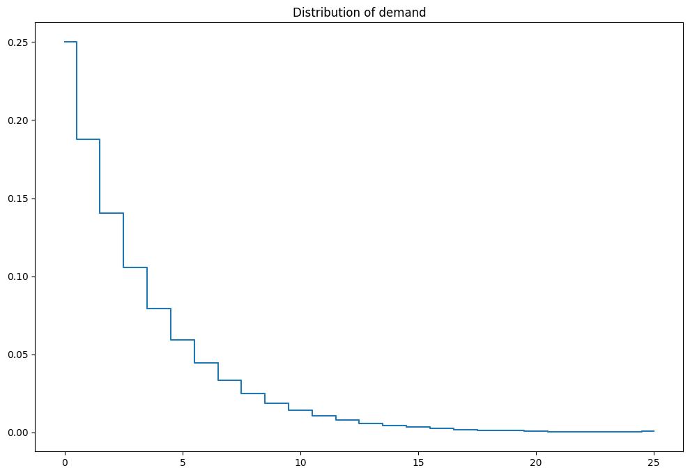
def demand_pr(self,plot=False):
'''Computes stochastic demand probs'''
k = np.arange(self.n) # all possible values of demand
pr = (1-self.dp)**k *self.dp
pr[-1] = 1 - pr[:-1].sum() # update last prob to ensure sum=1
if plot:
plt.step(self.x,pr,where='mid')
plt.title('Distribution of demand')
plt.show()
return pr
model=inventory_model(label='test')
print(model)
Inventory model labeled "test"
Paramters (c,p,r,β) = (3.2,2.5,0.5,0.95)
Demand=4
Upper bound on inventory 10
Show code cell source
def bellman(m,v0):
    '''Bellman equation for inventory model
        Inputs: model object
                next period value function
    '''
    # create the grid of choices (same as x), column-vector
    q = m.x[:,np.newaxis]
    # compute current period profit (relying on numpy broadcasting to get the matrix with choices in rows)
    p = m.profit(m.x,m.demand,q)
    # indexes for next period value with extrapolation using last value
    i = np.minimum(m.next_x(m.x,m.demand,q),m.upper)
    # compute the Bellman maximand
    vm = p + m.β*v0[i]
    # find max and argmax
    v1 = np.amax(vm,axis=0)   # maximum in every column
    q1 = np.argmax(vm,axis=0) # arg-maximum in every column = order volume
    return v1, q1

def solver_backwards_induction(m,T=10,verbose=False):
    '''Backwards induction solver for the finite horizon case'''
    # solution is time dependent
    m.value = np.zeros((m.n,T))
    m.policy = np.zeros((m.n,T))
    # main DP loop (from T to 1)
    for t in range(T,0,-1):
        if verbose:
            print('Time period %d\n'%t)
        j = t-1 # index of value and policy functions for period t
        if t==T:
            # terminal period: ordering zero is optimal
            m.value[:,j] = m.profit(m.x,m.demand,np.zeros(m.n))
            m.policy[:,j] = np.zeros(m.n)
        else:
            # all other periods
            m.value[:,j], m.policy[:,j] = bellman(m,m.value[:,j+1]) # next period to Bellman
        if verbose:
            print(m.value,'\n')
    # return model with updated value and policy functions
    return m
model = inventory_model(label='illustration')
model=solver_backwards_induction(model,T=5,verbose=True)
print('Optimal policy:\n',model.policy)
Time period 5

[[ 0.   0.   0.   0.   0. ]
 [ 0.   0.   0.   0.   2.5]
 [ 0.   0.   0.   0.   5. ]
 [ 0.   0.   0.   0.   7.5]
 [ 0.   0.   0.   0.  10. ]
 [ 0.   0.   0.   0.   9.5]
 [ 0.   0.   0.   0.   9. ]
 [ 0.   0.   0.   0.   8.5]
 [ 0.   0.   0.   0.   8. ]
 [ 0.   0.   0.   0.   7.5]
 [ 0.   0.   0.   0.   7. ]]

Time period 4

[[ 0.     0.     0.     4.3    0.   ]
 [ 0.     0.     0.     6.8    2.5  ]
 [ 0.     0.     0.     9.3    5.   ]
 [ 0.     0.     0.    11.8    7.5  ]
 [ 0.     0.     0.    14.3   10.   ]
 [ 0.     0.     0.    14.3    9.5  ]
 [ 0.     0.     0.    14.3    9.   ]
 [ 0.     0.     0.    15.625  8.5  ]
 [ 0.     0.     0.    17.5    8.   ]
 [ 0.     0.     0.    16.525  7.5  ]
 [ 0.     0.     0.    15.55   7.   ]]

Time period 3

[[ 0.     0.     9.425  4.3    0.   ]
 [ 0.     0.    11.925  6.8    2.5  ]
 [ 0.     0.    14.425  9.3    5.   ]
 [ 0.     0.    16.925 11.8    7.5  ]
 [ 0.     0.    19.425 14.3   10.   ]
 [ 0.     0.    19.425 14.3    9.5  ]
 [ 0.     0.    19.425 14.3    9.   ]
 [ 0.     0.    19.71  15.625  8.5  ]
 [ 0.     0.    21.585 17.5    8.   ]
 [ 0.     0.    21.085 16.525  7.5  ]
 [ 0.     0.    20.585 15.55   7.   ]]

Time period 2

[[ 0.      13.30575  9.425    4.3      0.     ]
 [ 0.      15.80575 11.925    6.8      2.5    ]
 [ 0.      18.30575 14.425    9.3      5.     ]
 [ 0.      20.80575 16.925   11.8      7.5    ]
 [ 0.      23.30575 19.425   14.3     10.     ]
 [ 0.      23.30575 19.425   14.3      9.5    ]
 [ 0.      23.30575 19.425   14.3      9.     ]
 [ 0.      24.57875 19.71    15.625    8.5    ]
 [ 0.      26.45375 21.585   17.5      8.     ]
 [ 0.      25.95375 21.085   16.525    7.5    ]
 [ 0.      25.45375 20.585   15.55     7.     ]]

Time period 1

[[17.9310625 13.30575    9.425      4.3        0.       ]
 [20.4310625 15.80575   11.925      6.8        2.5      ]
 [22.9310625 18.30575   14.425      9.3        5.       ]
 [25.4310625 20.80575   16.925     11.8        7.5      ]
 [27.9310625 23.30575   19.425     14.3       10.       ]
 [27.9310625 23.30575   19.425     14.3        9.5      ]
 [27.9310625 23.30575   19.425     14.3        9.       ]
 [28.2654625 24.57875   19.71      15.625      8.5      ]
 [30.1404625 26.45375   21.585     17.5        8.       ]
 [29.6404625 25.95375   21.085     16.525      7.5      ]
 [29.1404625 25.45375   20.585     15.55       7.       ]]

Optimal policy:
 [[8. 8. 8. 4. 0.]
 [8. 8. 8. 4. 0.]
 [8. 8. 8. 4. 0.]
 [8. 8. 8. 4. 0.]
 [8. 8. 8. 4. 0.]
 [7. 7. 7. 3. 0.]
 [6. 6. 6. 2. 0.]
 [0. 0. 0. 0. 0.]
 [0. 0. 0. 0. 0.]
 [0. 0. 0. 0. 0.]
 [0. 0. 0. 0. 0.]]
Show code cell source
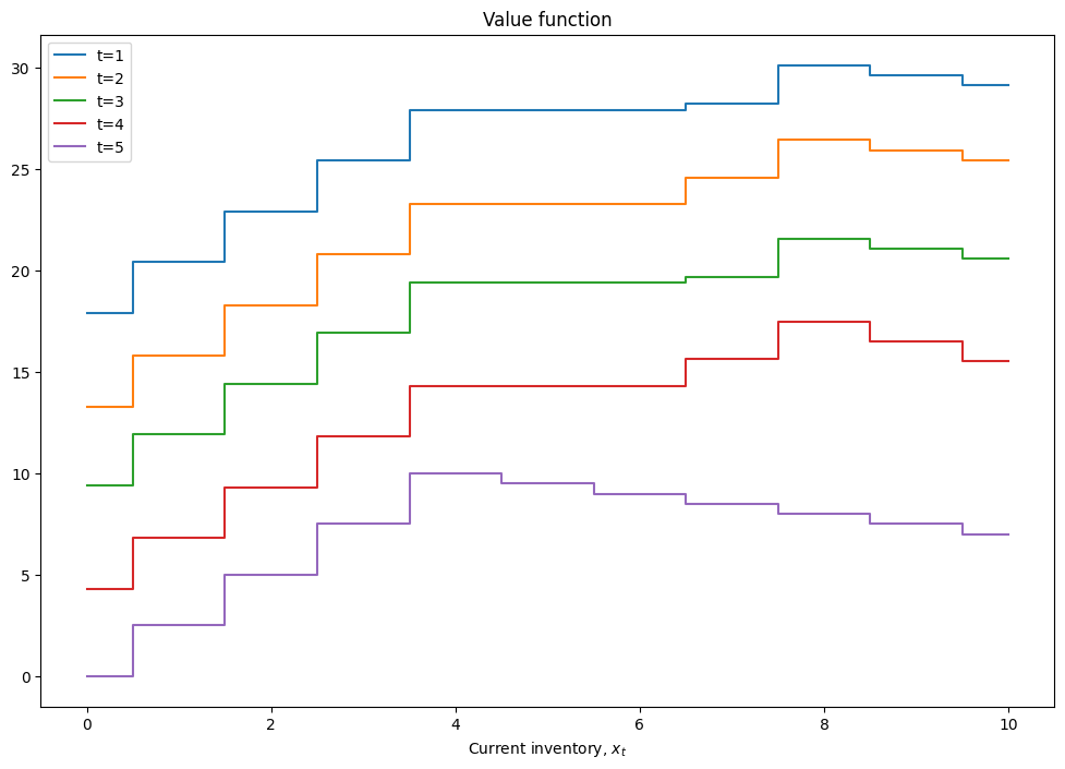
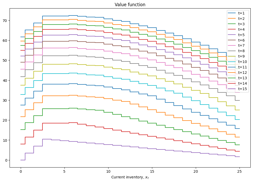
def plot_solution(model):
plt.step(model.x,model.value,where='mid')
plt.xlabel(r'Current inventory, $x_t$')
plt.legend([f't={i+1}' for i in range(model.value.shape[1])])
plt.title('Value function')
plt.show()
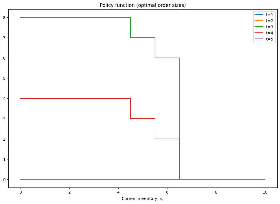
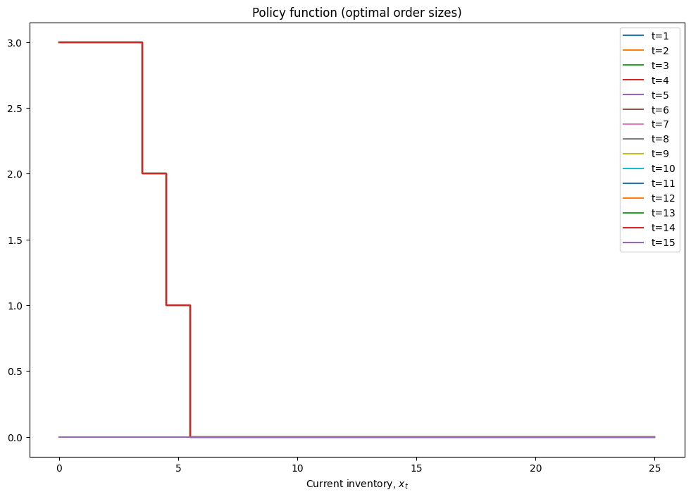
plt.step(model.x,model.policy,where='mid')
plt.xlabel(r'Current inventory, $x_t$')
plt.legend([f't={i+1}' for i in range(model.policy.shape[1])])
plt.title('Policy function (optimal order sizes)')
plt.show()
plot_solution(model)
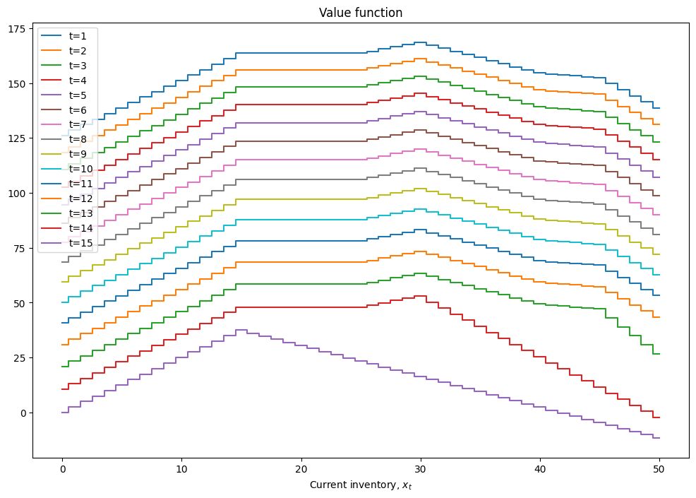
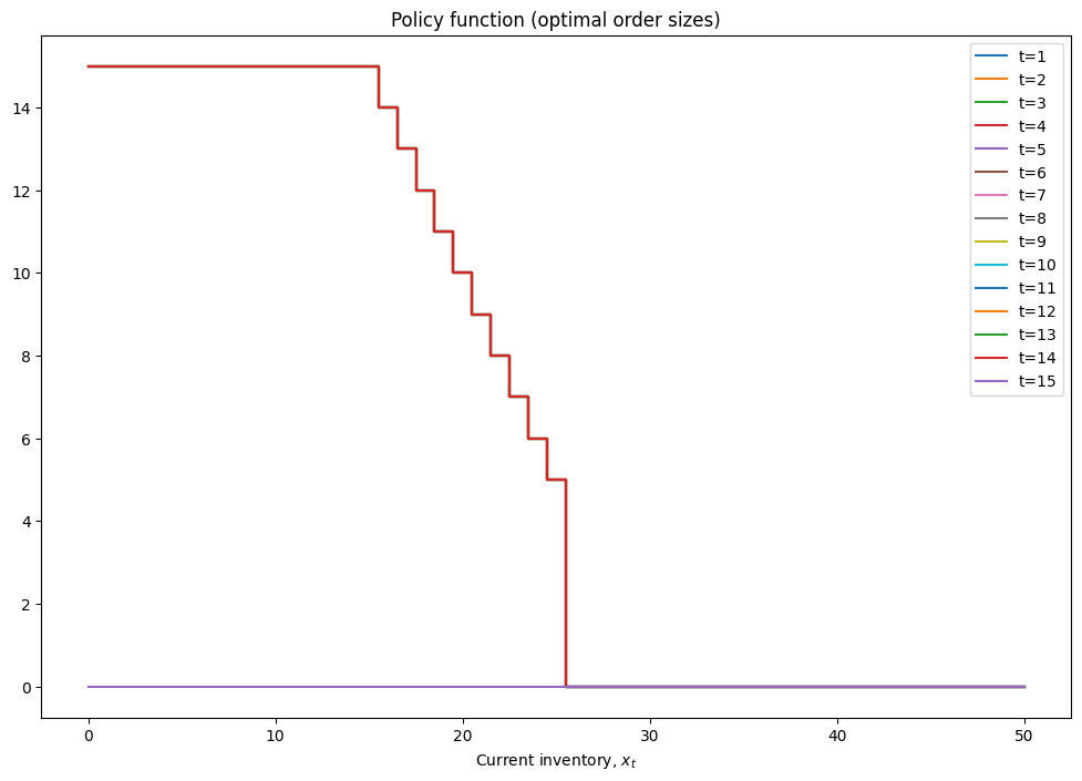
mod = inventory_model(label='production',max_inventory=50)
mod.demand = 15
mod.c = 5
mod.p = 2.5
mod.r = 1.4
mod.β = 0.975
mod = solver_backwards_induction(mod,T=15)
plot_solution(mod)
Note
Do we need to use backwards induction for the model above?
we could set it as a multivariate optimization w.r.t. the vector \((q_0,\dots,q_T)\)
the objective can be rewritten by plugging in the maximand of in period \(t+1\) into the equation for period \(t\) using the transition equation \(g(\cdot)\)
Thus any deterministic infinite horizon problem can be written and solved as a standard constrained optimization problem
But as soon as we introduce uncertainty, this approach breaks down:
there is no transition equation \(g(\cdot)\) to plug in, instead there is a transition probability and an expectation
the optimization problem in each period depends on the paramters (state variables) in a non-trivial way, and has to be solved separately for each value of parameters
Inventory management in infinite horizon#
Example
Return to the above example, now with the following modifications:
time horizon is infinite
demand is stochastic with known distribution
After dropping the time subscripts the Bellman equation is
The sum in the RHS of the equation computes the expectation over realizations of discrete random demands \(d'\), each happening with probability \(pr(d')\).
We could solve the problem as is, but note that \(d\) does not enter the “next period part” of the Bellman equation (due to the assumption that demand is idiosyncratic). In this case we can make our life easier by converting the problem of searching for the fixed point of the Bellman operator to the problem of searching the fixed point of the expected Bellman operator.
Taking the expectation of the Bellman equation over the distribution of demand \(d\) on both sides, and denoting \(EV(x) = \sum_{d} V(x,d) pr(d)\), we have
In the expected value function form the Bellman operator is also a contraction, but the fixed point now has to be solved only in the space of \(x\) and not \(x,d\). This is much easier for computational solver in the code below.
Show code cell source
def bellman_ev(m,ev0):
'''Bellman equation for inventory model
Inputs: model object
next period EXPECTED value function
'''
pr = m.demand_pr()
ev1 = np.zeros(shape=m.x.shape)
for j,d in enumerate(m.x): # over all values of demand
# create the grid of choices (same as x), column-vector
q = m.x[:,np.newaxis]
# compute current period profit (relying on numpy broadcasting to get the matrix with choices in rows)
p = m.profit(m.x,d,q)
# indexes for next period value with extrapolation using last value
i = np.minimum(m.next_x(m.x,d,q),m.upper)
# compute the Bellman maximand
vm = p + m.β*ev0[i]
# find max and argmax
v1 = np.amax(vm,axis=0) # maximum in every column
ev1 = ev1 + pr[j]*v1
q1 = None
return ev1, q1
def solve_vfi(self,tol=1e-6,maxiter=500,callback=None):
'''Solves the Rust model using value function iterations
'''
ev0 = np.zeros(self.n) # initial point for VFI
for i in range(maxiter): # main loop
ev1, q1 = bellman_ev(self,ev0) # update approximation
err = np.amax(np.abs(ev0-ev1))
if callback != None: callback(iter=i,err=err,ev1=ev1,ev0=ev0,q1=q1,model=self)
if err<tol:
break # break out if converged
ev0 = ev1 # get ready to the next iteration
else:
raise RuntimeError('Failed to converge in %d iterations'%maxiter)
return ev1, q1
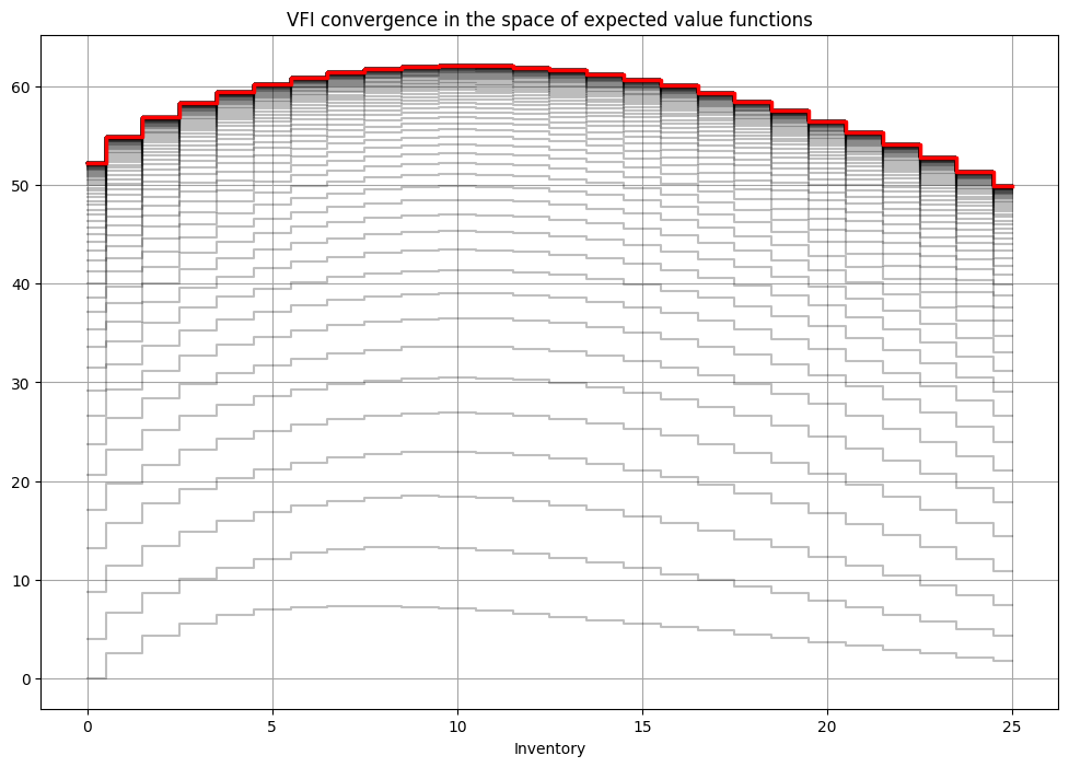
def solve_show(self,maxiter=1000,tol=1e-6,**kvargs):
'''Illustrate solution'''
fig1, (ax) = plt.subplots(1,1,figsize=(12,8))
ax.grid(which='both', color='0.65', linestyle='-')
ax.set_xlabel('Inventory')
ax.set_title('VFI convergence in the space of expected value functions')
def callback(**argvars):
mod, ev, q = argvars['model'],argvars['ev1'],argvars['q1']
ax.step(mod.x,ev,color='k',alpha=0.25,where='mid')
ev,pk = solve_vfi(self,maxiter=maxiter,tol=tol,callback=callback,**kvargs)
# add solutions
ax.step(self.x,ev,color='r',linewidth=2.5,where='mid')
plt.show()
def optimal_policy(m,ev):
'''Computes the optimal policy function for the stochastic
inventory dynamics model for given EV function'''
# idea: 3-dim array with q in axes 0, d in axis 1 and x in axis 2
q = m.x[:,np.newaxis,np.newaxis] # choices
d = m.x[np.newaxis,:,np.newaxis] # demand
x = m.x[np.newaxis,np.newaxis,:] # inventories
# compute current period profit (relying on numpy broadcasting to get the matrix with choices in rows)
p = m.profit(x,d,q) # 3-dim array
# indexes for next period value with extrapolation using last value
i = np.minimum(m.next_x(x,d,q),m.upper)
# compute the Bellman maximand
vm = p + m.β*ev[i]
# find argmax and argmax
return np.argmax(vm,axis=0) # maximum in every column
# Set up the parameters of the model
mod = inventory_model(label='production',max_inventory=25)
mod.dp=.25
mod.demand = int((1-mod.dp)/mod.dp) # mean for geometric distribution of demand
mod.c = .25
mod.p = 3.5
mod.r = 0.4
mod.β = 0.9

# solve the finite horizon version of the model with fixed demand
print(mod)
mod = solver_backwards_induction(mod,T=15)
plot_solution(mod)

# visualize the stochastic demand
mod.demand_pr(plot=True)

# solve the infinite horizon version of the model
ev,q = solve_vfi(mod)
solve_show(mod)
q = optimal_policy(mod,ev)
print('Optimal orders of new inventory for d,x:\n(d in rows, x in columns)')
print(q)
Inventory model labeled "production"
Paramters (c,p,r,β) = (0.25,3.5,0.4,0.9)
Demand=3
Upper bound on inventory 25
Optimal orders of new inventory for d,x:
(d in rows, x in columns)
[[7 6 5 4 3 2 0 0 0 0 0 0 0 0 0 0 0 0 0 0 0 0 0 0 0 0]
 [7 7 6 5 4 3 2 0 0 0 0 0 0 0 0 0 0 0 0 0 0 0 0 0 0 0]
 [7 7 7 6 5 4 3 2 0 0 0 0 0 0 0 0 0 0 0 0 0 0 0 0 0 0]
 [7 7 7 7 6 5 4 3 2 0 0 0 0 0 0 0 0 0 0 0 0 0 0 0 0 0]
 [7 7 7 7 7 6 5 4 3 2 0 0 0 0 0 0 0 0 0 0 0 0 0 0 0 0]
 [7 7 7 7 7 7 6 5 4 3 2 0 0 0 0 0 0 0 0 0 0 0 0 0 0 0]
 [7 7 7 7 7 7 7 6 5 4 3 2 0 0 0 0 0 0 0 0 0 0 0 0 0 0]
 [7 7 7 7 7 7 7 7 6 5 4 3 2 0 0 0 0 0 0 0 0 0 0 0 0 0]
 [7 7 7 7 7 7 7 7 7 6 5 4 3 2 0 0 0 0 0 0 0 0 0 0 0 0]
 [7 7 7 7 7 7 7 7 7 7 6 5 4 3 2 0 0 0 0 0 0 0 0 0 0 0]
 [7 7 7 7 7 7 7 7 7 7 7 6 5 4 3 2 0 0 0 0 0 0 0 0 0 0]
 [7 7 7 7 7 7 7 7 7 7 7 7 6 5 4 3 2 0 0 0 0 0 0 0 0 0]
 [7 7 7 7 7 7 7 7 7 7 7 7 7 6 5 4 3 2 0 0 0 0 0 0 0 0]
 [7 7 7 7 7 7 7 7 7 7 7 7 7 7 6 5 4 3 2 0 0 0 0 0 0 0]
 [7 7 7 7 7 7 7 7 7 7 7 7 7 7 7 6 5 4 3 2 0 0 0 0 0 0]
 [7 7 7 7 7 7 7 7 7 7 7 7 7 7 7 7 6 5 4 3 2 0 0 0 0 0]
 [7 7 7 7 7 7 7 7 7 7 7 7 7 7 7 7 7 6 5 4 3 2 0 0 0 0]
 [7 7 7 7 7 7 7 7 7 7 7 7 7 7 7 7 7 7 6 5 4 3 2 0 0 0]
 [7 7 7 7 7 7 7 7 7 7 7 7 7 7 7 7 7 7 7 6 5 4 3 2 0 0]
 [7 7 7 7 7 7 7 7 7 7 7 7 7 7 7 7 7 7 7 7 6 5 4 3 2 0]
 [7 7 7 7 7 7 7 7 7 7 7 7 7 7 7 7 7 7 7 7 7 6 5 4 3 2]
 [7 7 7 7 7 7 7 7 7 7 7 7 7 7 7 7 7 7 7 7 7 7 6 5 4 3]
 [7 7 7 7 7 7 7 7 7 7 7 7 7 7 7 7 7 7 7 7 7 7 7 6 5 4]
 [7 7 7 7 7 7 7 7 7 7 7 7 7 7 7 7 7 7 7 7 7 7 7 7 6 5]
 [7 7 7 7 7 7 7 7 7 7 7 7 7 7 7 7 7 7 7 7 7 7 7 7 7 6]
 [7 7 7 7 7 7 7 7 7 7 7 7 7 7 7 7 7 7 7 7 7 7 7 7 7 7]]
Note
Note the symmetry in the optimal policy! This implies that knowing both \(x\) and \(d\) is not necessary for the optional new order, it’s enough to condition on the inventory remaining after sales, i.e. \(x-\min(x,d) = \max(0,x-d)\)