Announcements & Reminders

1. Results of Online test 1

2. Orienteering at CBE on Wednesday March 13th, 12:00, behind CBE building. More information

📖 Sequences, limits and continuity

⏱ | words

Review of the basics of real analysis (mathematical analysis studies sequences, limit, continuity, differentiation, integration, etc.)

This lecture is on general theory of maxima and minima, and their existence.

• we have to cover a lot of ground, mostly somewhat familiar

• will work in \(\mathbb{R}^N\), the multidimensional space of real numbers 🤓

Plan:

1. Measuring distances in \(\mathbb{R}^N\) \(\rightarrow\) convergence

2. Bounded sets sets \(\rightarrow\) compact sets, existence of limits

3. Sequences \(\rightarrow\) convergence

4. Limits and convergences \(\rightarrow\) closedness

5. Open and closed sets \(\rightarrow\) compacts

6. Limits for functions \(\rightarrow\) continuity

7. Continuity of functions

8. Weierstrass extreme value theorem (continuous functions on compacts)

Note

Many textbooks use bold notation for vectors, but we do not. Typically it is explicitly stated that \(x \in \mathbb{R}^N\).

Norm and distance

Definition

The (Euclidean) norm of \(x \in \mathbb{R}^N\) is defined as

\[\| x \| = \left( \sum_{n=1}^N x_n^2 \right)^{1/2}\]

Interpretation:

• \(\| x \|\) represents the length of \(x\)

• \(\| x - y \|\) represents distance between \(x\) and \(y\)

Fig. 31 Length of red line \(= \sqrt{x_1^2 + x_2^2} =: \|x\|\)

\(\| x - y \|\) represents distance between \(x\) and \(y\)

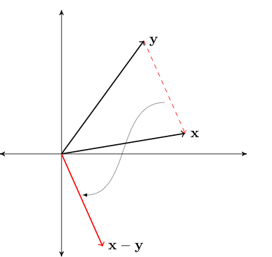
Fig. 32 Length of red line \(= \|x - y\|\)

Fact

For any \(\alpha \in \mathbb{R}\) and any \(x, y \in \mathbb{R}^N\), the following statements are true:

• \(\| x \| \geq 0\) and \(\| x \| = 0\) if and only if \(x = 0\)

• \(\| \alpha x \| = |\alpha| \| x \|\)

Triangle inequality

• \(\| x + y \| \leq \| x \| + \| y \|\)

Proof

For example, let’s show that \(\| x \| = 0 \iff x = 0\)

First let’s assume that \(\| x \| = 0\) and show \(x = 0\)

Since \(\| x \| = 0\) we have \(\| x \|^2 = 0\) and hence \(\sum_{n=1}^N x^2_n = 0\)

That is \(x_n = 0\) for all \(n\), or, equivalently, \(x = 0\)

Next let’s assume that \(x = 0\) and show \(\| x \| = 0\)

This is immediate from the definition of the norm

In fact, any function can be used as a norm, provided that the listed properties are satisfied

Example

More general distance function in \(\mathbb{R}\).

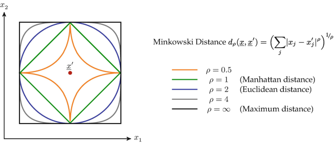
Fig. 33 Circle drawn with different norms

Naturally, in \(\mathbb{R}\) Euclidean norm simplifies to

\[\| x \| = \sqrt{x^2} = |x|\]

Show code cell source Hide code cell source

import numpy as np
import matplotlib.pyplot as plt

def subplots():
    "Custom subplots with axes throught the origin"
    fig, ax = plt.subplots()

    # Set the axes through the origin
    for spine in ['left', 'bottom']:
        ax.spines[spine].set_position('zero')
    for spine in ['right', 'top']:
        ax.spines[spine].set_color('none')
    
    ax.grid()
    return fig, ax

fig, ax = subplots()

ax.set_ylim(-3, 3)
ax.set_yticks((-3, -2, -1, 1, 2, 3))
x = np.linspace(-3, 3, 100)
ax.plot(x, np.abs(x), 'g-', lw=2, alpha=0.7, label=r'$f(x) = |x|$')
ax.plot(x, x, 'k--', lw=2, alpha=0.7, label=r'$f(x) = x$')
ax.legend(loc='lower right')

plt.show()

Therefore we can think of norm as a generalization of the absolute value to \(\mathbb{R}\)

Bounded sets

Definition

A set \(A \subset \mathbb{R}^N\) called bounded if

\[\exists \, M \in \mathbb{R} \; \mathrm{such\;that} \; \|x\| \leq M, \quad \forall \; x \in A\]

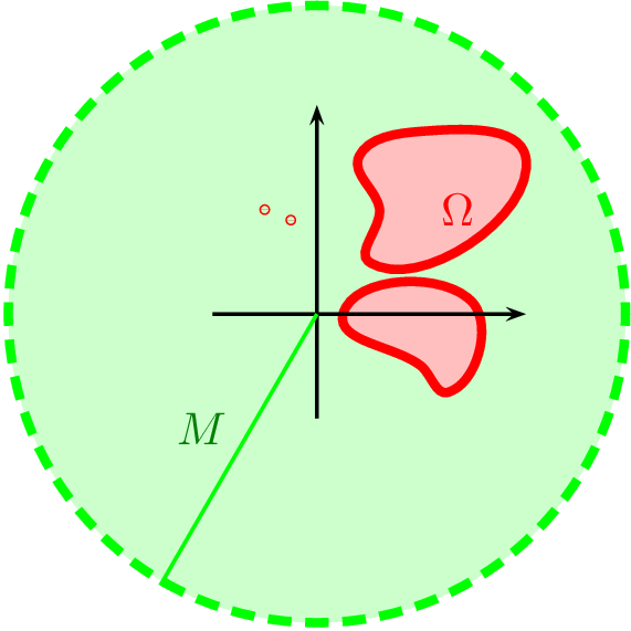
Fig. 34 Bounded set in \(\mathbb{R}^2\)

Example

Every finite subset \(A\) of \(\mathbb{R}\) is bounded

Indeed, set \(M := \max \{ |a| : a \in A \}\). Then \(A\) is bounded by definition

Example

The set \(\{(x,y)\in\mathbb{R}^2\colon xy \leqslant 1 \}\) is unbounded

Proof:

For any \(M \in \mathbb{R}\) consider the point whit coordinates \(x=1/M\) and \(y=M\). This point belongs to the set because it satisfies \(xy=1\), yet

\[\| (x,y) \| = \sqrt{x^2 + y^2} = \sqrt{\frac{1}{M^2} + M^2} > \sqrt{ M^2} = M\]

Therefore, for any candidate bound \(M\) we can find points in the set that are further away from the origin than \(M\).

Example

\((a, b)\) is bounded for any \(a, b \in \mathbb{R}\)

Proof:

Let \(M := \max\{ |a|, |b| \}\). We have to show that each \(x \in (a, b)\) satisfies \(|x| \leq M\)

\[x \in (a, b) \iff a < x < b\]

Cases:

1. \(0 \le a \le b \implies x > 0, x = |x| < |b| = b = \max\{|a|,|b|\}\)

2. \(a \le b \le 0 \implies a < x < 0, |x|= -x < -a = |a| = \max\{|a|,|b|\}\)

3. \(a \le 0 \le b \implies\)

\[\begin{split}\begin{cases} |x|<|b|, x \ge 0\\ |x|<|a|, x < 0 \end{cases} \implies |x|< \max\{|a|,|b|\} \text{ from 1. and 2.} $$\end{split}\]

Fact

If \(A\) and \(B\) are bounded sets then so is \(A \cup B\)

Proof

Let \(A\) and \(B\) be bounded sets and let \(C := A \cup B\)

By definition, \(\exists \, M_A\) and \(M_B\) with

\[\|a\| \leq M_A, \text{ all } a \in A, \quad \quad \|b\| \leq M_B, \text{ all } b \in B\]

Let \(M_C := \max\{M_A , M_B\}\) and fix any \(x \in C\)

\[x \in C \implies x \in A \text{ or } x \in B\]

\[\text{therefore } \|x\| \leq M_A \quad \text{or} \quad \|x\| \leq M_B\]

\[\text{therefore } \|x\| \leq M_C\]

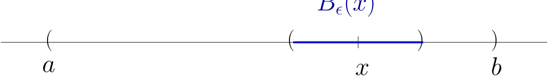
\(\epsilon\)-balls

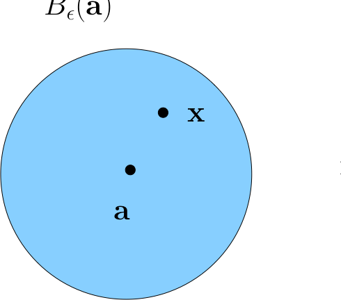
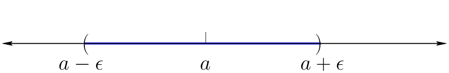
Definition

For \(\epsilon > 0\), the \(\epsilon\)-ball \(B_{\epsilon}(a)\) around \(a \in \mathbb{R}^N\) is all \(x \in \mathbb{R}^N\) such that \(\|a - x\| < \epsilon\)

Correspondingly, in one dimension \(\mathbb{R}\)

\[B_\epsilon(a) = \{ x \in \mathbb{R} : a - \epsilon < x < a + \epsilon \}\]

Fact

If \(x\) is in every \(\epsilon\)-ball around \(a\) then \(x=a\)

Proof

Suppose to the contrary that

• \(x\) is in every \(\epsilon\)-ball around \(a\) and yet \(x \ne a\)

Since \(x\) is not \(a\) we must have \(\|x-a\| > 0\)

Set \(\epsilon := \|x-a\|\)

Since \(\epsilon > 0\), we have \(x \in B_{\epsilon}(a)\)

This means that \(\|x-a\| < \epsilon\)

That is, \(\|x - a\| < \|x - a\|\)

Contradiction!

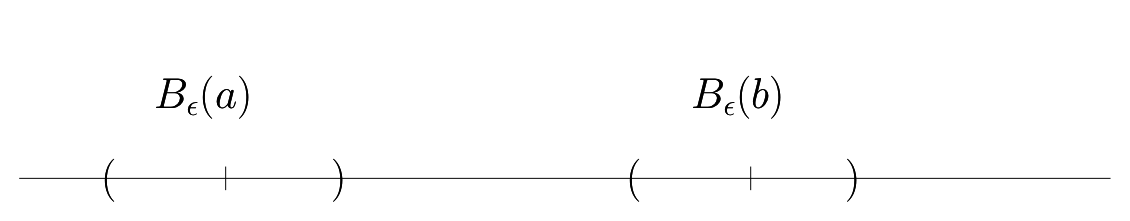
Fact

If \(a \ne b\), then \(\exists \; \epsilon > 0\) such that \(B_{\epsilon}(a)\) and \(B_{\epsilon}(b)\) are disjoint.

Proof

Let \(a, b \in \mathbb{R}^N\) with \(a \ne b\)

If we set \(\epsilon := \|a-b\|/2\), then \(B_{\epsilon}(a)\) and \(B_\epsilon(b)\) are disjoint

To see this, suppose to the contrary that \(\exists \, x \in B_{\epsilon}(a) \cap B_\epsilon(B)\)

Then \( \|x - a\| < \|a -b\|/2\) and \(\|x - b\| < \|a -b\|/2\)

But then

\[\|a - b\| \leq \|a - x\| + \|x - b\| < \|a -b\|/2 + \|a -b\|/2 = \|a-b\|\]

Contradiction!

Sequences

Definition

A sequence \(\{x_n\}\) in \(\mathbb{R}^N\) is a function from \(\mathbb{N}\) to \(\mathbb{R}^N\)

To each \(n \in \mathbb{N}\) we associate one \(x_n \in \mathbb{R}^N\)

Typically written as \(\{x_n\}_{n=1}^{\infty}\) or \(\{x_n\}\) or \(\{x_1, x_2, x_3, \ldots\}\)

Example

In \(\mathbb{R}\)

• \(\{x_n\} = \{2, 4, 6, \ldots \}\)

• \(\{x_n\} = \{1, 1/2, 1/4, \ldots \}\)

• \(\{x_n\} = \{1, -1, 1, -1, \ldots \}\)

• \(\{x_n\} = \{0, 0, 0, \ldots \}\)

In \(\mathbb{R}^N\)

• \(\{x_n\} = \big\{(2,..,2), (4,..,4), (6,..,6), \ldots \big\}\)

• \(\{x_n\} = \big\{(1, 1/2), (1/2,1/4), (1/4,1/8), \ldots \big\}\)

Definition

Sequence \(\{x_n\}\) is called bounded if \(\{x_1, x_2, \ldots\}\) is a bounded set.

Example

\[x_n = 1/n \quad x_n = (-1)^n \quad x_n = 2n\]

\[\text{(bounded)} \quad \text{(bounded)} \quad \text{(unbounded)}\]

Convergence and limit

\(\mathbb{R}^1\)

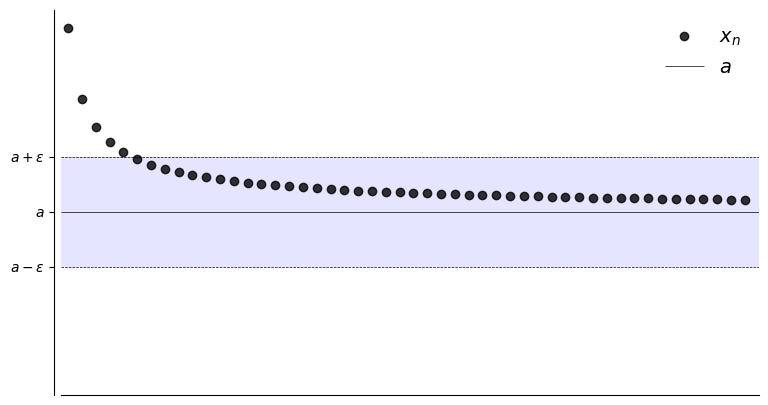
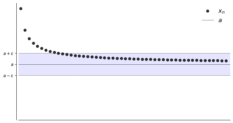
Let \(a \in \mathbb{R}\) and let \(\{x_n\}\) be a sequence

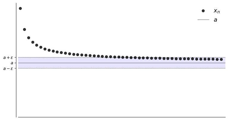
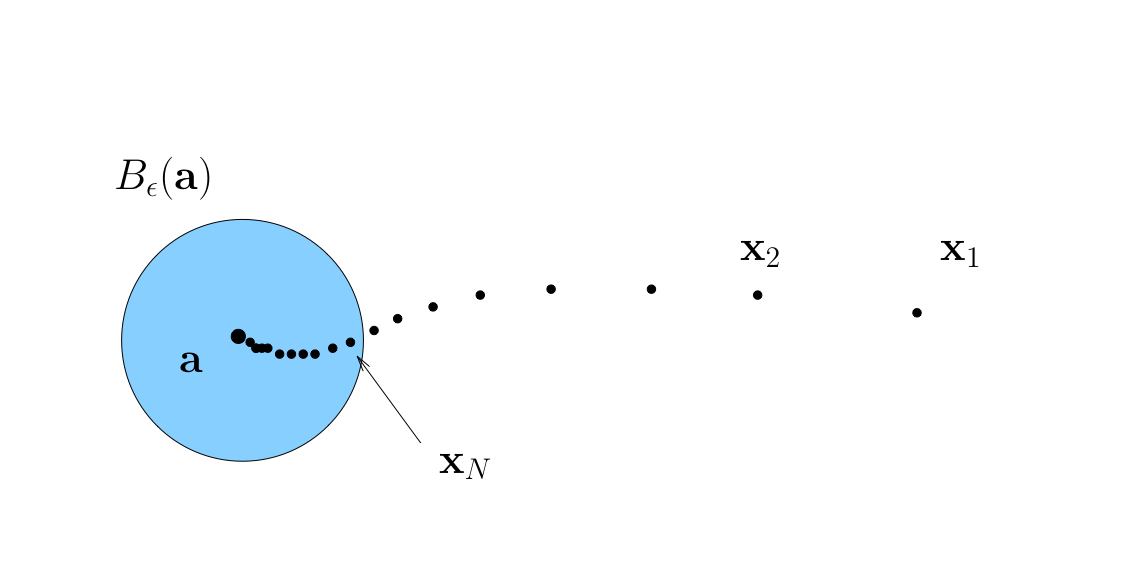
Suppose, for any \(\epsilon > 0\), we can find an \(N \in \mathbb{N}\) such that

\[x_n \in B_\epsilon(a) \text{ for all } n \geq N\]

alternatively for \(\mathbb{R}\)

\[| x_n -a | <\epsilon \text{ for all } n \geq N\]

Then \(\{x_n\}\) is said to converge to \(a\)

Convergence to \(a\) in symbols,

\[\forall \, \epsilon > 0, \; \exists \, N \in \mathbb{N} \; \text{ such that } n \geq N \implies x_n \in B_{\epsilon}(a)\]

The sequence \(\{x_n\}\) is eventually in this \(\epsilon\)-ball around \(a\)

Show code cell source Hide code cell source

import matplotlib.pyplot as plt
import numpy as np

# from matplotlib import rc
# rc('font',**{'family':'serif','serif':['Palatino']})
# rc('text', usetex=True)

def fx(n):
    return 1 + 1/(n**(0.7))
def subplots(fs):
    "Custom subplots with axes throught the origin"
    fig, ax = plt.subplots(figsize=fs)
    # Set the axes through the origin
    for spine in ['left', 'bottom']:
        ax.spines[spine].set_position('zero')
    for spine in ['right', 'top']:
        ax.spines[spine].set_color('none')
    return fig, ax
def plot_seq(N,epsilon,a,fn):
    fig, ax = subplots((9, 5))  
    xmin, xmax = 0.5, N+1
    ax.set_xlim(xmin, xmax)
    ax.set_ylim(0, 2.1)
    n = np.arange(1, N+1)
    ax.set_xticks([])
    ax.plot(n, fn(n), 'ko', label=r'$x_n$', alpha=0.8)
    ax.hlines(a, xmin, xmax, color='k', lw=0.5, label='$a$')
    ax.hlines([a - epsilon, a + epsilon], xmin, xmax, color='k', lw=0.5, linestyles='dashed')
    ax.fill_between((xmin, xmax), a - epsilon, a + epsilon, facecolor='blue', alpha=0.1)
    ax.set_yticks((a - epsilon, a, a + epsilon))
    ax.set_yticklabels((r'$a - \epsilon$', r'$a$', r'$a + \epsilon$'))
    ax.legend(loc='upper right', frameon=False, fontsize=14)
    plt.show()

N = 50
a = 1
plot_seq(N,0.30,a,fx)
plot_seq(N,0.20,a,fx)
plot_seq(N,0.10,a,fx)

Definition

The point \(a\) is called the limit of the sequence, denoted

\[x_n \to a \text{ as } n \to \infty \quad \text{ or } \quad \lim_{n \to \infty} x_n = a,\]

if

\[\forall \, \epsilon > 0, \; \exists \, N \in \mathbb{N} \; \text{ such that } n \geq N \implies |x_n - a|< \epsilon\]

Example

\(\{x_n\}\) defined by \(x_n = 1 + 1/n\) converges to \(1\):

\[x_n \to 1 \; \mathrm{as} \; n \to \infty \quad\text{or}\quad \lim_{n \to \infty} x_n = 1\]

To prove this we must show that \(\forall \, \epsilon > 0\), there is an \(N \in \mathbb{N}\) such that

\[n \geq N \implies |x_n - 1| < \epsilon\]

To show this formally we need to come up with an “algorithm”

1. You give me any \(\epsilon > 0\)

2. I respond with an \(N\) such that equation above holds

In general, as \(\epsilon\) shrinks, \(N\) will have to grow

Proof:

Here’s how to do this for the case \(1 + 1/n\) converges to \(1\)

First pick an arbitrary \(\epsilon > 0\)

Now we have to come up with an \(N\) such that

\[n \geq N \implies |1 + 1/n - 1| < \epsilon\]

Let \(N\) be the first integer greater than \( 1/\epsilon\)

Then

\[n \geq N \implies n > 1/\epsilon \implies 1/n < \epsilon \implies |1 + 1/n - 1| < \epsilon \]

Remark: Any \(N' > N\) would also work

Example

The sequence \(x_n = 2^{-n}\) converges to \(0\) as \(n \to \infty\)

Proof:

Must show that, \(\forall \, \epsilon > 0\), \(\exists \, N \in \mathbb{N}\) such that

\[n \geq N \implies |2^{-n} - 0| < \epsilon\]

So pick any \(\epsilon > 0\), and observe that

\[|2^{-n} - 0| < \epsilon \; \iff \; 2^{-n} < \epsilon \; \iff \; n > - \frac{\ln \epsilon}{\ln 2}\]

Hence we take \(N\) to be the first integer greater than \(- \ln \epsilon / \ln 2\)

Then

\[n \geq N \implies n > -\frac{\ln \epsilon}{\ln 2} \implies |2^{-n} - 0| < \epsilon\]

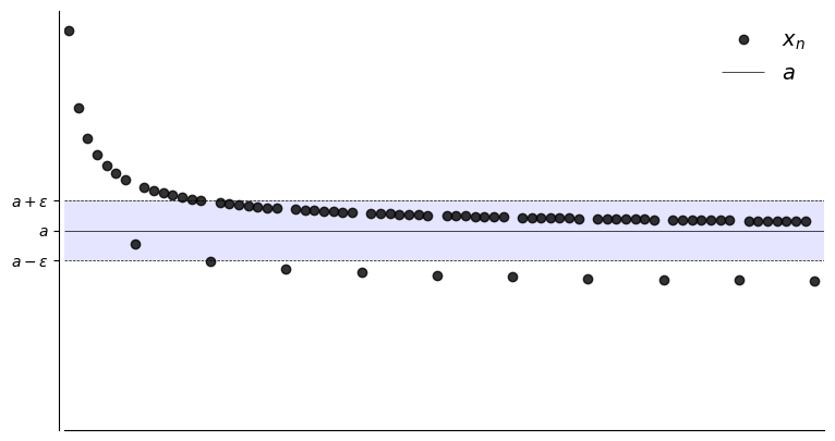
What if we want to show that \(x_n \to a\) fails?

To show convergence fails we need to show the negation of

\[\forall \,\; \epsilon > 0, \;\; \exists \,\; N \in \mathbb{N} \;\mathrm{such\;that}\; n \geq N \implies x_n \in B_{\epsilon}(a)\]

In words, there is an \(\epsilon > 0\) where we can’t find any such \(N\)

That is, for any choice of \(N\) there will be \(n>N\) such that \(x_n\) jumps to the outside \(B_{\epsilon}(a)\)

In other words, there exists a \(B_\epsilon(a)\) such that \(x_n \notin B_\epsilon(a)\) again and again as \(n \to \infty\).

This is the kind of picture we’re thinking of

Show code cell source Hide code cell source

def fx2(n):
    return 1 + 1/(n**(0.7)) - 0.3 * (n % 8 == 0)

N = 80
a = 1
plot_seq(N,0.15,a,fx2)

Example

The sequence \(x_n = (-1)^n\) does not converge to any \(a \in \mathbb{R}\)

Proof:

This is what we want to show

\[\exists \,\; \epsilon > 0 \;\text{ such that } x_n \notin B_{\epsilon}(a) \text{ infinitely many times as } n \to \infty\]

Since it’s a “there exists”, we need to come up with such an \(\epsilon\)

Let’s try \(\epsilon = 0.5\), so that

\[B_\epsilon(a) = \{ x \in \mathbb{R} : |x - a| < 0.5 \} = (a-0.5, a+0.5 )\]

We have:

• If \(n\) is odd then \(x_n = -1\) when \(n > N\) for any \(N\).

• If \(n\) is even then \(x_n = 1\) when \(n > N\) for any \(N\).

Therefore even if \(a=1\) or \(a=-1\), \(\{x_n\}\) not in \(B_\epsilon(a)\) infinitely many times as \(n \to \infty\). It holds for all other values of \(a \in \mathbb{R}\).

\(\mathbb{R}^N\)

Definition

Sequence \(\{x_n\}\) is said to converge to \(a \in \mathbb{R}^N\) if

\[\forall \epsilon > 0, \; \exists \, N \in \mathbb{N} \; \text{ such that } \; n \geq N \implies x_n \in B_{\epsilon}(a)\]

We can say

\(\{x_n\}\) is eventually in any \(\epsilon\)-neighborhood of \(a\)

In this case \(a\) is called the limit of the sequence, and as in one-dimensional case, we write

\[x_n \to a \; \text{ as } \; n \to \infty \quad \text{or} \quad \lim_{n \to \infty} x_n = a\]

Definition

We call \(\{ x_n \}\) convergent if it converges to some limit in \(\mathbb{R}^N\)

Vector vs Componentwise Convergence

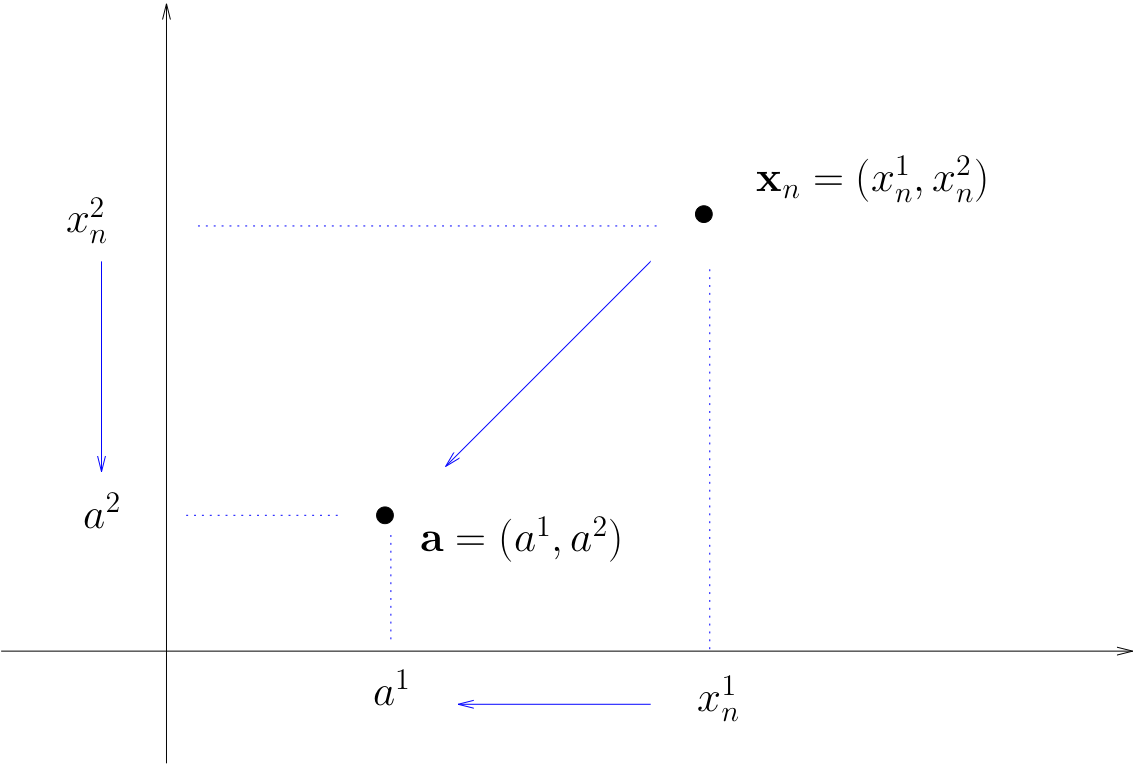
Fact

A sequence \(\{x_n\}\) in \(\mathbb{R}^N\) converges to \(a \in \mathbb{R}^N\) if and only if each component sequence converges in \(\mathbb{R}\)

That is,

\[\begin{split}\begin{pmatrix} x^1_n \\ \vdots \\ x^K_n \end{pmatrix} \to \begin{pmatrix} a^1 \\ \vdots \\ a^K \end{pmatrix} \quad \text{in } \mathbb{R}^N \quad \iff \quad \begin{array}{cc} x^1_n \to a^1 & \quad \text{in } \mathbb{R} \\ \vdots & \\ x^K_n \to a^K & \quad \text{in } \mathbb{R} \end{array}\end{split}\]

Proof

The sketch of the proof:

• \(\Rightarrow\) (necessity): verify that the definition of convergence in \(\mathbb{R}\) corresponds to the convergence in each dimension by definition where \(\epsilon\)-neighborhoods are projection of the \(B_\epsilon(a)\)

• \(\Leftarrow\) (sufficiency): verify that convergence in \(\mathbb{R}\) by definition follows from the definitions to the convergence in each dimension when the required \(B_\epsilon(a)\) ball is constructed to contain the hypercube of the \(\epsilon\)-neighborhoods of each dimension.

Properties of limit

Fact

1. \(x_n \to a\) in \(\mathbb{R}^N\) if and only if \(\|x_n - a\| \to 0\) in \(\mathbb{R}\)

2. If \(x_n \to x\) and \(y_n \to y\) then \(x_n + y_n \to x + y\)

3. If \(x_n \to x\) and \(\alpha \in \mathbb{R}\) then \(\alpha x_n \to \alpha x\)

4. If \(x_n \to x\) and \(y_n \to y\) then \(x_n y_n \to xy\)

5. If \(x_n \to x\) and \(y_n \to y\) then \(x_n / y_n \to x/y\), provided \(y_n \ne 0\), \(y \ne 0\)

6. If \(x_n \to x\) then \(x_n^p \to x^p\)

Proof

Let’s prove that

\[x_n \to a \text{ in } \mathbb{R}^N \; \iff \; \|x_n - a\| \to 0 \text{ in } \mathbb{R}\]

• \(x_n \to a\) in \(\mathbb{R}^N\) means that

\[\forall \, \epsilon > 0, \; \exists \, N \in \mathbb{N} \; \mathrm{such\;that} \; n \geq N \implies \| x_n - a \| < \epsilon\]

• \(\|x_n - a\| \to 0\) in \(\mathbb{R}\) means that

\[\forall\, \epsilon > 0, \; \exists \, N \in \mathbb{N} \; \mathrm{such\;that} \; n \geq N \implies | \| x_n - a \| - 0 | < \epsilon\]

Obviously equivalent

Exercise: Prove other properties using definition of limit

Fact

Each sequence in \(\mathbb{R}^N\) has at most one limit

Proof

Proof for the \(\mathbb{R}\) case.

Suppose instead that \(x_n \to a \text{ and } x_n \to b \text{ with } a \ne b \)

Take disjoint \(\epsilon\)-balls around \(a\) and \(b\)

Since \(x_n \to a\) and \(x_n \to b\),

• \(\exists \; N_a\) s.t. \(n \geq N_a \implies x_n \in B_{\epsilon}(a)\)

• \(\exists \; N_b\) s.t. \(n \geq N_b \implies x_n \in B_{\epsilon}(b)\)

But then \(n \geq \max\{N_a, N_b\} \implies \) \(x_n \in B_{\epsilon}(a)\) and \(x_n \in B_{\epsilon}(b)\)

Contradiction, as the balls are assumed disjoint

Fact

Every convergent sequence is bounded

Proof

Proof for the \(\mathbb{R}\) case.

Let \(\{x_n\}\) be convergent with \(x_n \to a\)

Fix any \(\epsilon > 0\) and choose \(N\) s.t. \(x_n \in B_{\epsilon}(a)\) when \(n \geq N\)

Regarded as sets,

\[\{x_n\} \subset \{x_1, \ldots, x_{N-1}\} \cup B_{\epsilon}(a)\]

Both of these sets are bounded

• First because finite sets are bounded

• Second because \(B_{\epsilon}(a)\) is bounded

Further, finite unions of bounded sets are bounded

Cauchy sequences

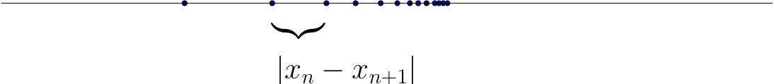
Informal definition: Cauchy sequences are those where \(|x_n - x_{n+1}|\) gets smaller and smaller

Example

Sequences generated by iterative methods for solving nonlinear equations often have this property

Show code cell source Hide code cell source

f = lambda x: -4*x**3+5*x+1
g = lambda x: -12*x**2+5

def newton(fun,grad,x0,tol=1e-6,maxiter=100,callback=None):
    '''Newton method for solving equation f(x)=0
    with given tolerance and number of iterations.
    Callback function is invoked at each iteration if given.
    '''
    for i in range(maxiter):
        x1 = x0 - fun(x0)/grad(x0)
        err = abs(x1-x0)
        if callback != None: callback(err=err,x0=x0,x1=x1,iter=i)
        if err<tol: break
        x0 = x1
    else:
        raise RuntimeError('Failed to converge in %d iterations'%maxiter)
    return (x0+x1)/2

def print_err(iter,err,**kwargs):
    x = kwargs['x'] if 'x' in kwargs.keys() else kwargs['x0']
    print('{:4d}:  x = {:14.8f}    diff = {:14.10f}'.format(iter,x,err))

print('Newton method')
res = newton(f,g,x0=123.45,callback=print_err,tol=1e-10)

Newton method
   0:  x =   123.45000000    diff =  41.1477443465
   1:  x =    82.30225565    diff =  27.4306976138
   2:  x =    54.87155804    diff =  18.2854286376
   3:  x =    36.58612940    diff =  12.1877193931
   4:  x =    24.39841001    diff =   8.1212701971
   5:  x =    16.27713981    diff =   5.4083058492
   6:  x =    10.86883396    diff =   3.5965889909
   7:  x =     7.27224497    diff =   2.3839931063
   8:  x =     4.88825187    diff =   1.5680338561
   9:  x =     3.32021801    diff =   1.0119341175
  10:  x =     2.30828389    diff =   0.6219125117
  11:  x =     1.68637138    diff =   0.3347943714
  12:  x =     1.35157701    diff =   0.1251775194
  13:  x =     1.22639949    diff =   0.0188751183
  14:  x =     1.20752437    diff =   0.0004173878
  15:  x =     1.20710698    diff =   0.0000002022
  16:  x =     1.20710678    diff =   0.0000000000

Definition

A sequence \(\{x_n\}\) is called Cauchy if

\[\forall \; \epsilon > 0, \;\; \exists \; N \in \mathbb{N} \; \mathrm{such\;that}\; \forall n, m \geqslant N \implies \| x_n - x_m \| < \epsilon\]

Alternatively

\[\forall \; \epsilon > 0, \;\; \exists \; N \in \mathbb{N} \; \mathrm{such\;that}\; \forall j \geqslant N \implies \| x_n - x_{n+j} \| < \epsilon\]

Cauchy sequences allow to establish convergence without finding the limit itself!

Fact

Every convergent sequence is Cauchy, and every Cauchy sequence is convergent.

Proof

Proof of \(\Rightarrow\):

Let \(\{x_n\}\) be a sequence converging to some \(a \in \mathbb{R}\)

Fix \(\epsilon > 0\)

We can choose \(N\) s.t.

\[n \geq N \;\; \implies \;\; |x_n - a | < \frac{\epsilon}{2} \]

For this \(N\) we have \(n \geq N\) and \(j \geq 1\) implies

\[|x_n - x_{n+j}| \leq |x_n - a| + |x_{n+j} - a| < \frac{\epsilon}{2} + \frac{\epsilon}{2} = \epsilon\]

Proof of \(\Leftarrow\):

Follows from the density property of \(\mathbb{R}\)

Example

\(\{x_n\}\) defined by \(x_n = \alpha^n\) where \(\alpha \in (0, 1)\) is Cauchy

Proof:

For any \(n , j\) we have

\[|x_n - x_{n+j}| = |\alpha^n - \alpha^{n+j}| = \alpha^n |1 - \alpha^j| \leq \alpha^n\]

Fix \(\epsilon > 0\)

We can show that \(n > \log(\epsilon) / \log(\alpha) \implies \alpha^n < \epsilon\)

Hence any integer \(N > \log(\epsilon) / \log(\alpha)\) the sequence is Cauchy by definition.

Subsequences

Definition

A sequence \(\{x_{n_k} \}\) is called a subsequence of \(\{x_n\}\) if

1. \(\{x_{n_k} \}\) is a subset of \(\{x_n\}\)

2. \(\{n_k\}\) is sequence of strictly increasing natural numbers

Example

\[\{x_n\} = \{x_1, x_2, x_3, x_4, x_5, \ldots\} \]

\[\{x_{n_k}\} = \{x_2, x_4, x_6, x_8 \ldots\} \]

In this case

\[\{n_k\} = \{n_1, n_2, n_3, \ldots\} = \{2, 4, 6, \ldots\}\]

Example

\(\{\frac{1}{1}, \frac{1}{3}, \frac{1}{5},\ldots\}\) is a subsequence of \(\{\frac{1}{1}, \frac{1}{2}, \frac{1}{3}, \ldots\}\)

\(\{\frac{1}{1}, \frac{1}{2}, \frac{1}{3},\ldots\}\) is a subsequence of \(\{\frac{1}{1}, \frac{1}{2}, \frac{1}{3}, \ldots\}\)

\(\{\frac{1}{2}, \frac{1}{2}, \frac{1}{2},\ldots\}\) is not a subsequence of \(\{\frac{1}{1}, \frac{1}{2}, \frac{1}{3}, \ldots\}\)

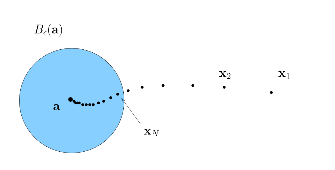
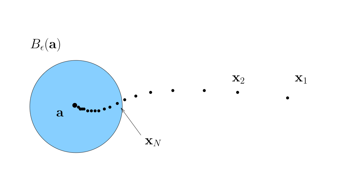
Fact

If \(\{ x_n \}\) converges to \(x\) in \(\mathbb{R}^N\), then every subsequence of \(\{x_n\}\) also converges to \(x\)

Fig. 35 Convergence of subsequences

Bolzano-Weierstrass theorem

This leads us to the famous theorem, which will be part of the proof of the central Weierstrass extreme values theorem, which provides conditions for existence of a maximum and minimum of a function.

Fact: Bolzano-Weierstrass theorem

Every bounded sequence in \(\mathbb{R}^N\) has a convergent subsequence

Proof

Omitted, but see Wiki and resources referenced there.

Open and closed sets

Definition

Let \(G \subset \mathbb{R}^N\). We call \(x \in G\) interior to \(G\) if \(\exists \; \epsilon > 0\) with \(B_\epsilon(x) \subset G\)

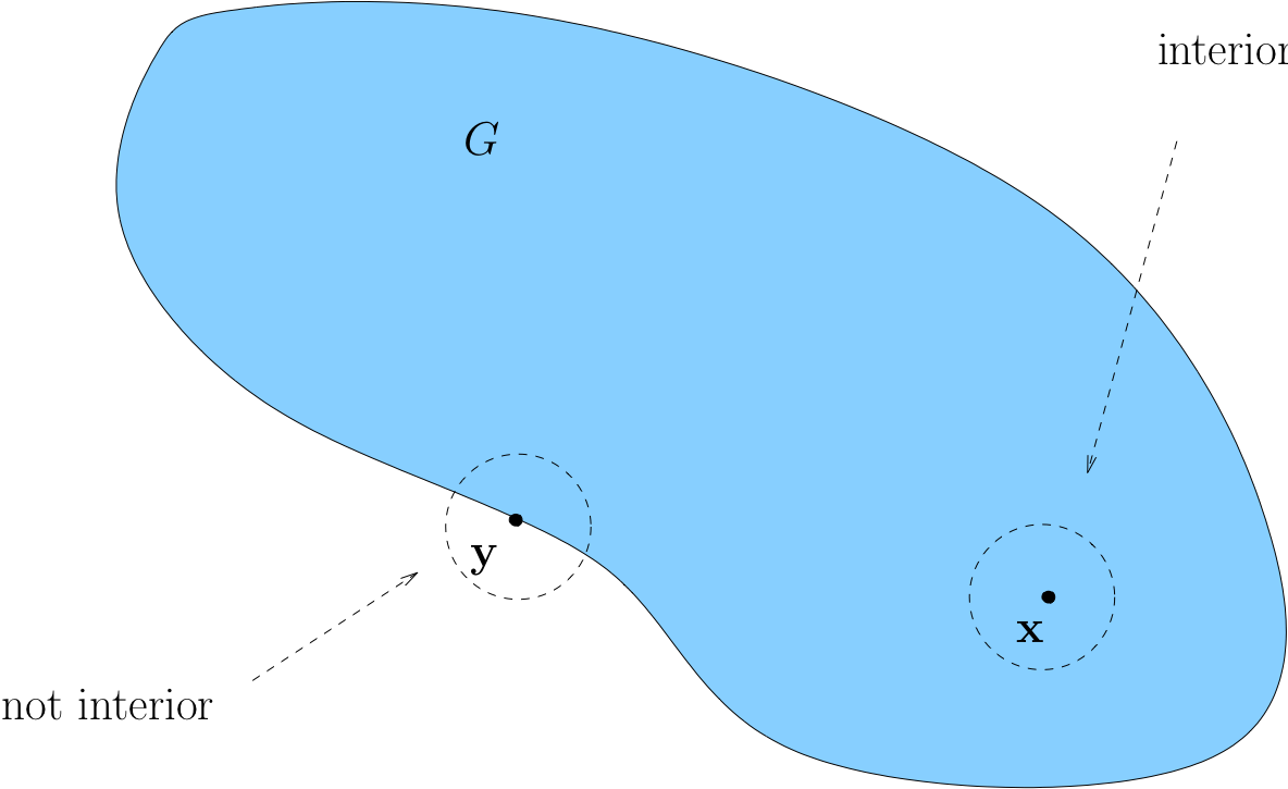
Fig. 36 Loosely speaking, interior means “not on the boundary”

Example

Example

If \(G = (a, b)\) for some \(a < b\), then any \(x \in (a, b)\) is interior

Proof:

Fix any \(a < b\) and any \(x \in (a, b)\)

Let \(\epsilon := \min\{x - a, b - x\}\)

If \(y \in B_\epsilon(x)\) then \(y < b\) because

\[y = y + x - x \leq |y - x| + x < \epsilon + x \leq b - x + x = b\]

Exercise: Show \(y \in B_\epsilon(x) \implies y > a\)

Example

If \(G = [-1, 1]\), then \(1\) is not interior

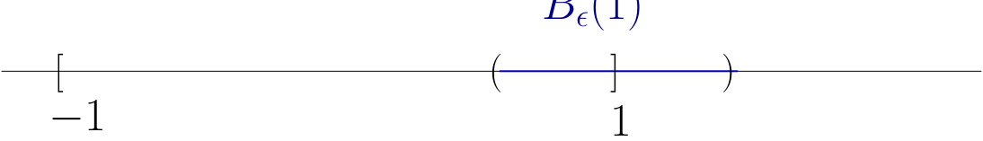
Proof:

Intuitively, any \(\epsilon\)-ball centered on \(1\) will contain points \(> 1\)

More formally, pick any \(\epsilon > 0\) and consider \(B_\epsilon(1)\)

There exists a \(y \in B_\epsilon(1)\) such that \(y \notin [-1, 1]\)

For example, consider the point \(y := 1 + \epsilon/2\)

Exercise: Check this point: lies in \(B_\epsilon(1)\) but not in \([-1, 1]\)

Definition

A set \(G\subset \mathbb{R}^N\) is called open if all of its points are interior

Example

Open sets:

• any open interval \((a,b) \subset \mathbb{R}\), since we showed all points are interior

• any open ball \(B_\epsilon(a) = x \in \mathbb{R}^N : \|x - a \| < \epsilon\)

• \(\mathbb{R}^N\) itself satisfies the defintion of open set

Sets that are not open

• \((a,b]\) because \(b\) is not interior

• \([a,b)\) because \(a\) is not interior

Closed Sets

Definition

A set \(F \subset \mathbb{R}^N\) is called closed if every convergent sequence in \(F\) converges to a point in \(F\)

Rephrased: If \(\{x_n\} \subset F\) and \(x_n \to x\) for some \(x \in \mathbb{R}^N\), then \(x \in F\)

Example

All of \(\mathbb{R}^N\) is closed \(\Leftarrow\) every sequence converging to a point in \(\mathbb{R}^N\) converges to a point in \(\mathbb{R}^N\)!

Example

If \((-1, 1) \subset \mathbb{R}\) is not closed

Proof:

True because

1. \(x_n := 1-1/n\) is a sequence in \((-1, 1)\) converging to \(1\),

2. and yet \(1 \notin (-1, 1)\)

Example

If \(F = [a, b] \subset \mathbb{R}\) then \(F\) is closed in \(\mathbb{R}\)

Proof:

Take any sequence \(\{x_n\}\) such that

• \(x_n \in F\) for all \(n\)

• \(x_n \to x\) for some \(x \in \mathbb{R}\)

We claim that \(x \in F\)

Recall that (weak) inequalities are preserved under limits:

• \(x_n \leq b\) for all \(n\) and \(x_n \to x\), so \(x \leq b\)

• \(x_n \geq a\) for all \(n\) and \(x_n \to x\), so \(x \geq a\)

therefore \(x \in [a, b] =: F\)

Properties of Open and Closed Sets

Fact

\(G \subset \mathbb{R}^N\) is open \(\iff \; G^c\) is closed

Proof

\(\implies\)

First prove necessity

Pick any \(G\) and let \(F := G^c\)

Suppose to the contrary that \(G\) is open but \(F\) is not closed, so

\(\exists\) a sequence \(\{x_n\} \subset F\) with limit \(x \notin F\)

Then \(x \in G\), and since \(G\) open, \(\exists \, \epsilon > 0\) such that \(B_\epsilon(x) \subset G\)

Since \(x_n \to x\) we can choose an \(N \in \mathbb{N}\) with \(x_N \in B_\epsilon(x)\)

This contradicts \(x_n \in F\) for all \(n\)

\(\Longleftarrow\)

Next prove sufficiency

Pick any closed \(F\) and let \(G := F^c\), need to prove that \(G\) is open

Suppose to the contrary that \(G\) is not open

Then exists some non-interior \(x \in G\), that is no \(\epsilon\)-ball around \(x\) lies entirely in \(G\)

Then it is possible to find a sequence \(\{x_n\}\) which converges to \(x \in G\), but every element of which lies in the \(B_{1/n}(x) \cap F\)

This contradicts the fact that \(F\) is closed

Fact

Any singleton \(\{ x \} \subset \mathbb{R}^N\) is closed

Proof

Let’s prove this by showing that \(\{x\}^c\) is open

Pick any \(y \in \{x\}^c\)

We claim that \(y\) is interior to \(\{x\}^c\)

Since \(y \in \{x\}^c\) it must be that \(y \ne x\)

Therefore, exists \(\epsilon > 0\) such that \(B_\epsilon(y) \cap B_\epsilon(x) = \varnothing\)

In particular, \(x \notin B_\epsilon(y)\), and hence \(B_\epsilon(y) \subset \{x\}^c\)

Therefore \(y\) is interior as claimed

Since \(y\) was arbitrary it follows that \(\{x\}^c\) is open and \(\{x\}\) is closed

Fact

1. Any finite union of open sets is open

2. Any finite intersection of closed sets is closed

Proof

Proof of first fact:

Let \(G := \cup_{\lambda \in \Lambda} G_\lambda\), where each \(G_\lambda\) is open

We claim that any given \(x \in G\) is interior to \(G\)

Pick any \(x \in G\)

By definition, \(x \in G_\lambda\) for some \(\lambda\)

Since \(G_\lambda\) is open, \(\exists \, \epsilon > 0\) such that \(B_\epsilon(x) \subset G_\lambda\)

But \(G_\lambda \subset G\), so \(B_\epsilon(x) \subset G\) also holds

In other words, \(x\) is interior to \(G\)

But be careful:

• An infinite intersection of open sets is not necessarily open

• An infinite union of closed sets is not necessarily closed

For example, if \(G_n := (-1/n, 1/n)\), then \(\cap_{n \in \mathbb{N}} G_n = \{0\} \)

Definition

Set \(X\) is called compact if it is both closed and bounded.

Continuity of functions

Fundamental property of functions, required not only to establish existence of optima and optimizers, but also roots, fixed points, etc.

Definition

Let \(f \colon A \in \mathbb{R}^N \to \mathbb{R}\)

\(f\) is called continuous at \(x \in A\) if

\[\forall \{x_n\} \in A \colon \lim_{n \to \infty} x_n = x \in A \quad \implies \quad f(x_n) \to f(x) \]

Note that the definition requires that

• \(f(x_n)\) converges for each choice of \(x_n \to x\),

• the limit is always the same, and that limit is \(f(x)\)

Definition

\(f: A \to \mathbb{R}\) is called continuous if it is continuous at every \(x \in A\)

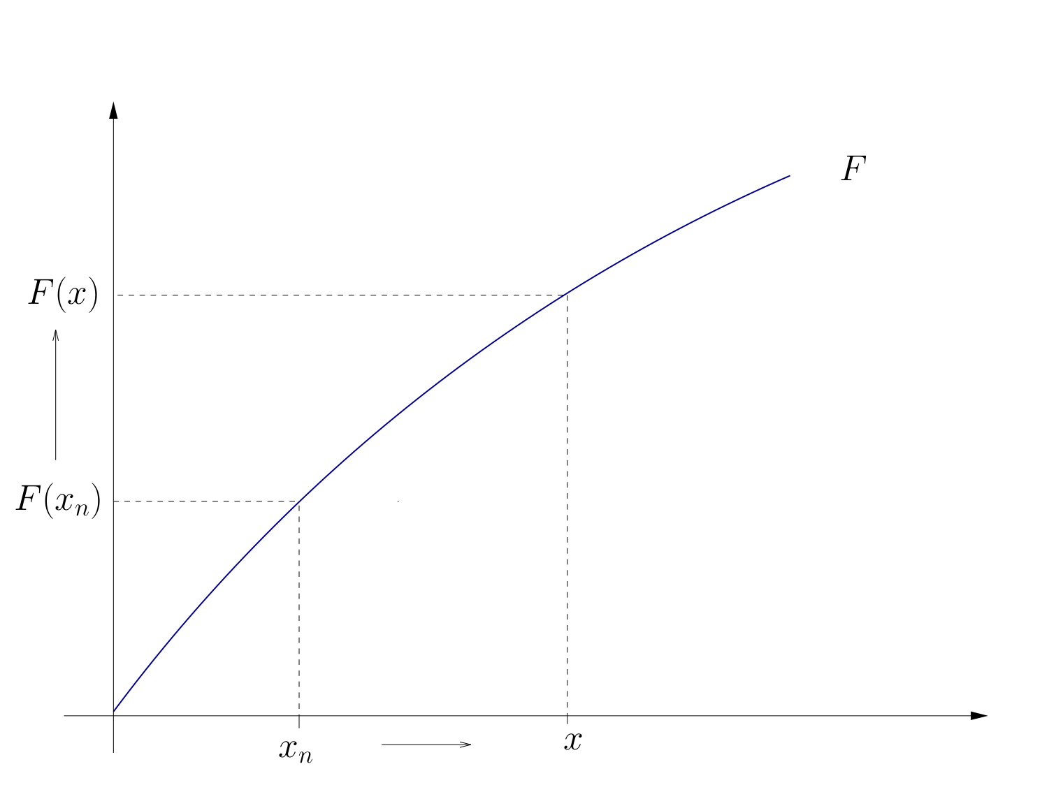
Fig. 37 Continuous function

Example

Function \(f(x) = \exp(x)\) is continuous at \(x=0\)

Proof:

Consider any sequence \(\{x_n\}\) which converges to \(0\)

We want to show that for any \(\epsilon>0\) there exists \(N\) such that \(n \geq N \implies |f(x_n) - f(0)| < \epsilon\). We have

\[\begin{split}\begin{array}{l} |f(x_n) - f(0)| = |\exp(x_n) - 1| < \epsilon \quad \iff \\ \exp(x_n) - 1 < \epsilon \; \text{ and } \; \exp(x_n) - 1 > -\epsilon \quad \iff \\ x_n < \ln(1+\epsilon) \; \text{ and } \; x_n > \ln(1-\epsilon) \quad \Longleftarrow \\ | x_n - 0 | < \min \big(\ln(1+\epsilon),\ln(1-\epsilon) \big) = \ln(1-\epsilon) \end{array}\end{split}\]

Because due to \(x_n \to x\) for any \(\epsilon' = \ln(1-\epsilon)\) there exists \(N\) such that \(n \geq N \implies |x_n - 0| < \epsilon'\), we have \(f(x_n) \to f(x)\) by definition. Thus, \(f\) is continuous at \(x=0\).

Fact

Some functions known to be continuous on their domains:

• \(f: x \mapsto x^\alpha\)

• \(f: x \mapsto |x|\)

• \(f: x \mapsto \log(x)\)

• \(f: x \mapsto \exp(x)\)

• \(f: x \mapsto \sin(x)\)

• \(f: x \mapsto \cos(x)\)

Types of discontinuities

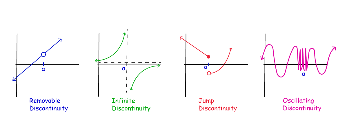
Fig. 38 4 common types of discontinuity

Example

The indicator function \(x \mapsto \mathbb{1}\{x > 0\}\) has a jump discontinuity at \(0\).

Fact

Let \(f\) and \(g\) be functions and let \(\alpha \in \mathbb{R}\)

1. If \(f\) and \(g\) are continuous at \(x\) then so is \(f + g\), where

\[(f + g)(x) := f(x) + g(x)\]

2. If \(f\) is continuous at \(x\) then so is \(\alpha f\), where

\[(\alpha f)(x) := \alpha f(x)\]

3. If \(f\) and \(g\) are continuous at \(x\) and real valued then so is \(f \circ g\), where

\[(f \circ g)(x) := f(x) \cdot g(x)\]

In the latter case, if in addition \(g(x) \ne 0\), then \(f/g\) is also continuous.

Proof

Just repeatedly apply the properties of the limits

Let’s just check that

\[\text{$f$ and $g$ continuous at $x$} \implies \text{$f + g$ continuous at $x$}\]

Let \(f\) and \(g\) be continuous at \(x\)

Pick any \(x_n \to x\)

We claim that \(f(x_n) + g(x_n) \to f(x) + g(x)\)

By assumption, \(f(x_n) \to f(x)\) and \(g(x_n) \to g(x)\)

From this and the triangle inequality we get

\[\| f(x_n) + g(x_n) - (f(x) + g(x)) \| \leq \]

\[\leq \| f(x_n) - f(x) \| + \| g(x_n) - g(x) \| \to 0\]

As a result, set of continuous functions is “closed” under elementary arithmetic operations

Example

The function \(f \colon \mathbb{R} \to \mathbb{R}\) defined by

\[f(x) = \frac{\exp(x) + \sin(x)}{2 + \cos(x)} + \frac{x^4}{2} - \frac{\cos^3(x)}{8!}\]

is continuous (we just have to be careful to ensure that denominator is not zero – which it is not for all \(x\in\mathbb{R}\))

Example

An example of oscillating discontinuity is the function \(f(x) = \sin(1/x)\) which is discontinuous at \(x=0\).

Video to illustrate this function

Weierstrass boundedness theorem

Putting together all the above material to formulate a fundamental result which is essential for establishing the existence of maxima and minima of functions in the next section.

Definition

A function \(f\) is called bounded if its range is a bounded set.

Fact

Consider a continuous function \(f: X \subset \mathbb{R}^N \to \mathbb{R}\).

If \(X\) is compact, then \(f\) is bounded on \(X\).

Proof

Sketch of the proof:

• Suppose that range of \(f\) denoted \(f(X)\) is not a bounded set

• Then we can find a sequence \(\{x_n\}\) in \(X\) such \(\forall n\in\mathbb{N}\) there exists \(f(x_n)\) such that \(|f(n)|>n\).

• Sequence \(\{x_n\}\) is bounded, so by Bolzano-Weierstrass theorem it has a convergent subsequence \(\{x_{n_k}\}\), where \(n_k\) is a subset of \(\mathbb{N}\) index by \(k\), and thus \(k \leqslant n_k\) for all \(k\)

• Denote by \(L\) the limit of this subsequence, \(L = \lim_{k \to \infty} \{x_{n_k}\}\)

• \(L \in X\) because \(X\) is a compact and thus is a closed set

• By continuity of \(f\) at \(L\) we have that \(f(x_{n_k}) \to f(L)\)

• Then the sequence \(\{f(x_{n_k})\}\) is bounded due to the properties of the limit (see above)

• This contradicts that by our construction \(|f(x_n)| > n \geqslant k\) where \(k\) can be arbitrary large

Also see the discussion here

Notes from the lecture

Hand written notes from the lecture

References and further reading

References

• Simon & Blume: 12.1, 12.2, 12.3, 12.4, 12.5 10.1, 10.2, 10.3, 10.4, 13.4

• Sundaram: 1.1.1, 1.1.2, 1.2.1, 1.2.2, 1.2.3, 1.2.7, 1.2.8, 1.4.1

Further reading and self-learning

Watch excellent video by Grant Sanderson (3blue1brown) on limits, and continue onto his whole amazing series on calculus