🔬 Tutorial problems lambda

Show code cell content Hide code cell content

import numpy as np
import matplotlib.pyplot as plt
from mpl_toolkits.mplot3d import Axes3D
from matplotlib import cm
from myst_nb import glue

f = lambda x: (x[0])**3 - (x[1])**3
lb,ub = -1.5,1.5

x = y = np.linspace(lb,ub, 100)
X, Y = np.meshgrid(x, y)
zs = np.array([f((x,y)) for x,y in zip(np.ravel(X), np.ravel(Y))])
Z = zs.reshape(X.shape)

a,b=1,1
# (x/a)^2 + (y/b)^2 = 1
theta = np.linspace(0, 2 * np.pi, 100)
X1 = a*np.cos(theta)
Y1 = b*np.sin(theta)
zs = np.array([f((x,y)) for x,y in zip(np.ravel(X1), np.ravel(Y1))])
Z1 = zs.reshape(X1.shape)

fig = plt.figure(dpi=160)
ax2 = fig.add_subplot(111)
ax2.set_aspect('equal', 'box')
ax2.contour(X, Y, Z, 50,
            cmap=cm.jet)
ax2.plot(X1, Y1)
plt.setp(ax2, xticks=[],yticks=[])
glue("pic1", fig, display=False)

fig = plt.figure(dpi=160)
ax3 = fig.add_subplot(111, projection='3d')
ax3.plot_wireframe(X, Y, Z,
            rstride=2,
            cstride=2,
            alpha=0.7,
            linewidth=0.25)
f0 = f(np.zeros((2)))+0.1
ax3.plot(X1, Y1, Z1, c='red')
plt.setp(ax3,xticks=[],yticks=[],zticks=[])
ax3.view_init(elev=18, azim=154)
glue("pic2", fig, display=False)


f = lambda x: x[0]**3/3 - 3*x[1]**2 + 5*x[0] - 6*x[0]*x[1]
x = y = np.linspace(-10.0, 10.0, 100)
X, Y = np.meshgrid(x, y)
zs = np.array([f((x,y)) for x,y in zip(np.ravel(X), np.ravel(Y))])
Z = zs.reshape(X.shape)
a,b=4,8
# (x/a)^2 + (y/b)^2 = 1
theta = np.linspace(0, 2 * np.pi, 100)
X1 = a*np.cos(theta)
Y1 = b*np.sin(theta)
zs = np.array([f((x,y)) for x,y in zip(np.ravel(X1), np.ravel(Y1))])
Z1 = zs.reshape(X1.shape)

fig = plt.figure(dpi=160)
ax2 = fig.add_subplot(111)
ax2.set_aspect('equal', 'box')
ax2.contour(X, Y, Z, 50,
            cmap=cm.jet)
ax2.plot(X1, Y1)
plt.setp(ax2, xticks=[],yticks=[])
glue("pic3", fig, display=False)

fig = plt.figure(dpi=160)
ax3 = fig.add_subplot(111, projection='3d')
ax3.plot_wireframe(X, Y, Z, 
            rstride=2, 
            cstride=2,
            alpha=0.7,
            linewidth=0.25)
f0 = f(np.zeros((2)))+0.1
ax3.plot(X1, Y1, Z1, c='red')
plt.setp(ax3,xticks=[],yticks=[],zticks=[])
ax3.view_init(elev=18, azim=154)
glue("pic4", fig, display=False)

\(\lambda\).1

Formulation

Solve the following constrained maximization problem using the Karush-Kuhn-Tucker method. Verify that the found stationary/critical points satisfy the second order conditions.

\[\begin{split} \begin{array}{c} f(x,y) = x^3 - y^3 \to \max_{x,y}\\ \text {subject to} \\ x^2 + y^2 \le 1,\\ x,y \in \mathbb{R} \end{array} \end{split}\]

Hint

Standard KKT method should work for this problem.

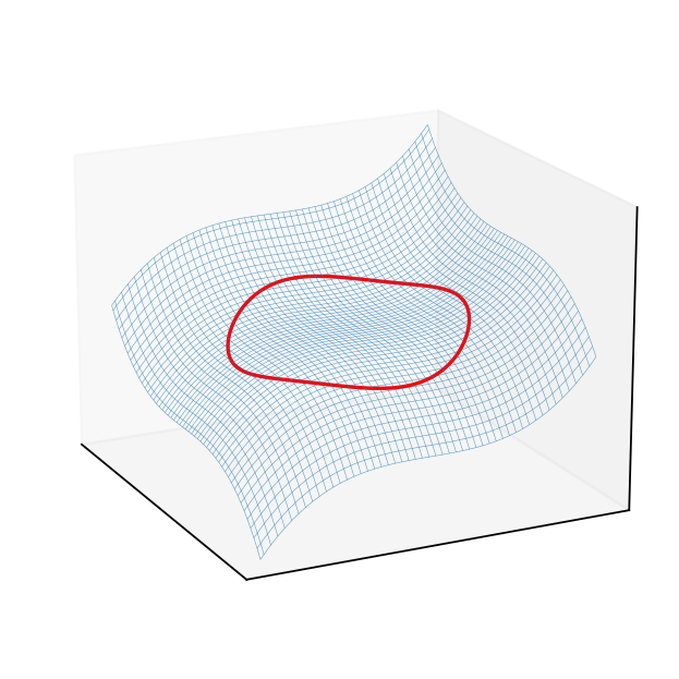
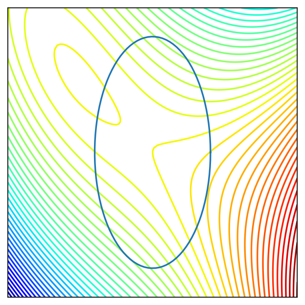
Fig. 100 Level curves of the criterion function and constraint curve.

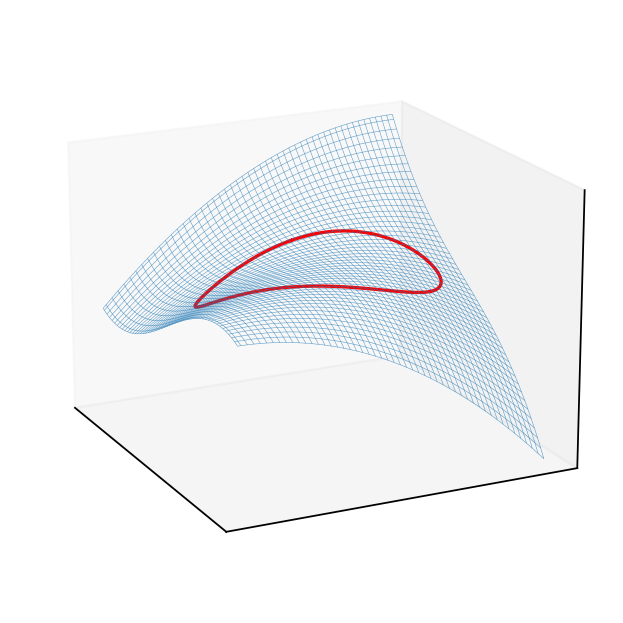
Fig. 101 3D plot of the criterion surface with the constraint curve projected to it.

Solution

The constraint is \(g(x,y) := x^2-y^2 - 1 \le 0\). The Lagrangian function is

\[ \mathcal{L}(x,y,\lambda) = x^3-y^3- \lambda (x^2 + y^2-1) \]

The necessary KKT conditions are given by the following system of equations and inequalities

\[\begin{split} \begin{array}{rl} \frac{\partial \mathcal{L}}{\partial x} =& 3x^2 - 2 \lambda x=0\\ \frac{\partial \mathcal{L}}{\partial y} =& -3 y^2 -2 \lambda y=0 \\ & x^2- y^2-1 \le 0 \\ & \lambda \ge 0 \\ & \lambda g(x,y) = \lambda (x^2- y^2-1) = 0 \end{array} \end{split}\]

To solve this system, we start from checking the two possible cases: \(\lambda=0\) and \(\lambda>0\).

Case 1. \(\lambda=0\): the constraint could not be binding. Then, the FOCs imply \(x=y=0\). The unconstrained Hessian matrix is

\[\begin{split} Hf(0,0) = \begin{pmatrix} \frac{\partial^2 f}{\partial x^2} & \frac{\partial^2 f}{\partial x \partial y} \\ \frac{\partial^2 f}{\partial y \partial x} & \frac{\partial^2 f}{\partial y^2} \end{pmatrix}_{(x,y)=(0,0)} = \begin{pmatrix} 6x & 0\\ 0 & -6y \end{pmatrix}_{(x,y)=(0,0)} = \begin{pmatrix} 0 & 0\\ 0 & 0 \end{pmatrix}_{(x,y)=(0,0)} \end{split}\]

We have \(\det(H)=0\) and \(trace(H)=0\) so that there is no sufficient information to conclude the property of the stationary point.

Case 2. \(\lambda>0\): the constraint is binding. Then, the problem is the optimization with equality constraint, given two control variables \(N=2\) and one constraint \(K=1\). From the FOCs, we have

\[\begin{split} \begin{array}{l} 0=3x^2 - 2 \lambda x= x(3x -2\lambda) \Longrightarrow x=0, \text{ or } x = \frac{2}{3}\lambda\\ 0=-3 y^2 -2 \lambda y= y(-3y-2\lambda) \Longrightarrow y=0, \text{ or } y = -\frac{2}{3}\lambda \end{array} \end{split}\]

Since further we have the constraint \(x^2+y^2=1\), there are three cases: “\(x=0, y<0\)”, “\(x>0, y=0\)” or “\(x>0, y<0\)”.

(i) If \(x>0, y<0\), then it follows from the above conditions that

\[\begin{split} \frac{3}{2}x =\lambda = -\frac{3}{2}y \\ \implies y=-x. \end{split}\]

Since \(x^2+y^2=1\) and \(x>0, y<0\), we have \(x=1/\sqrt{2}, y=-1/\sqrt{2}\) and then \(\lambda= 3/(2\sqrt{2})\).

Observe that \(\mathrm{rank}(Dg)) = \mathrm{rank}((2x, 2y)) = 1\) for \(x \ne 0\) or \(y\neq0\), so the constrained qualification holds for any point on the boundary.

The bordered Hessian matrix is

\[\begin{split} H \mathcal{L}(x,y,\lambda)) = \begin{pmatrix} 0 & \frac{\partial^2 \mathcal{L}}{\partial \lambda \partial x} & \frac{\partial^2 \mathcal{L}}{\partial \lambda \partial y}\\ \frac{\partial^2 \mathcal{L}}{\partial \lambda \partial x}& \frac{\partial^2 \mathcal{L}}{\partial x^2} & \frac{\partial^2 \mathcal{L}}{\partial y \partial x} \\ \frac{\partial^2 \mathcal{L}}{\partial \lambda \partial y}& \frac{\partial^2 \mathcal{L}}{\partial x \partial y} & \frac{\partial^2 \mathcal{L}}{\partial y^2} \end{pmatrix} = \begin{pmatrix} 0& -2x& -2y \\ -2x& 6x -2\lambda & 0\\ -2y& 0&-6y -2\lambda \end{pmatrix}. \end{split}\]

Now, the bordered Hessian at \((x,y,\lambda) = (1/\sqrt{2}, -1/\sqrt{2}, 3/(2\sqrt{2}))\) is

\[\begin{split} H \mathcal{L} (1/\sqrt{2}, -1/\sqrt{2}, 3/(2\sqrt{2}))= \begin{pmatrix} 0& -\sqrt{2}& \sqrt{2} \\ -\sqrt{2}& 3\sqrt{2} -3/\sqrt{2} & 0\\ \sqrt{2}& 0& 3\sqrt{2} -3/\sqrt{2} \end{pmatrix}. \end{split}\]

It suffices to check the last leading principal minor. The determinant is

\[\begin{split} \det (H \mathcal{L} (1/\sqrt{2}, -1/\sqrt{2}, 3/(2\sqrt{2})) = -(-\sqrt{2})\begin{vmatrix} -\sqrt{2}& \sqrt{2} \\ 0& 3\sqrt{2} -3/\sqrt{2} \end{vmatrix} + \sqrt{2}\begin{vmatrix} -\sqrt{2}& \sqrt{2} \\ 3\sqrt{2} -3/\sqrt{2} & 0 \end{vmatrix}\\ = -6\sqrt{2} < 0, \end{split}\]

which has the same sign as \((-1)^K=(-1)\). Therefore, it is positive definite and we have a local minimum on the boundary.

(ii) If \(x=0, y<0\), then from \(x^2+y^2=1\), we have \(y=-1\). Also, \(\lambda=-3y/2 = 3/2\). The border Hessian is

\[\begin{split} H \mathcal{L}(0,-1,\frac{3}{2})) = \begin{pmatrix} 0& -2x& -2y \\ -2x& 6x -2\lambda & 0\\ -2y& 0&-6y -2\lambda \end{pmatrix} = \begin{pmatrix} 0&0& 2\\ 0& -3 &0\\ 2&0 & 3 \end{pmatrix}. \end{split}\]

The determinant is \(\det (H\mathcal{L})=12 >0\), which has the same sign as \((-1)^2\) and then the Hessian matrix is negative definite. Therefore, \((0, -1)\) is a local maximum.

(iii) If \(x>0, y=0\), then from \(x^2+y^2=1\), we have \(x=1\). Also, \(\lambda=3x/2 = 3/2\). The border Hessian is

\[\begin{split} H \mathcal{L}(1,0,\frac{3}{2})) = \begin{pmatrix} 0& -2x& -2y \\ -2x& 6x -2\lambda & 0\\ -2y& 0&-6y -2\lambda \end{pmatrix} = \begin{pmatrix} 0&-2& 0\\ -2& 3 &0\\ 0&0 & -3 \end{pmatrix}. \end{split}\]

The determinant is \(\det (H\mathcal{L})=12 >0\), which has the same sign as \((-1)^2\) and then the Hessian matrix is negative definite. Therefore, \((1, 0)\) is a local maximum.

Finally, the objective values for the local maximums are \(f(1,0)=f(0,-1)=1\) and note that the constrained set is compact. Therefore, these two local maximizers are also global maximizers.

\(\lambda\).2

Formulation

Solve the following constrained maximization problem using the Karush-Kuhn-Tucker method. Verify that the found stationary/critical points satisfy the second order conditions.

\[\begin{split} \begin{array}{c} f(x,y) = -x^2 \to \max_{x,y} \\ \text {subject to} \\ x^2-y^2-2xy \ge 2,\\ x,y \in \mathbb{R} \end{array} \end{split}\]

Hint

Standard KKT method should work for this problem.

Solution

The Lagrangian function is

\[ \mathcal{L}(\lambda,x,y) = -x^2 - \lambda (-x^2 + y^2 +2xy + 2) \]

KKT conditions are

\[\begin{split} \left\{ \begin{array}{rl} \frac{\partial \mathcal{L}}{\partial x} &= -2x + 2\lambda x - 2\lambda y = 0,\\ \frac{\partial \mathcal{L}}{\partial y} &= - 2\lambda y - 2\lambda x = 0,\\ & -x^2 + y^2 +2xy + 2 \le 0,\\ & \lambda \ge 0,\\ & \lambda (-x^2 + y^2 +2xy + 2) = 0. \end{array} \right. \end{split}\]

Case 1: \(\lambda = 0\)

This is the unconstrained case with the number of variables \(N=2\). KKT conditions simplify to

\[\begin{split} \left\{ \begin{array}{l} -2x = 0,\\ -x^2 + y^2 +2xy + 2 \le 0 \end{array} \right. \end{split}\]

Thus, \(x=0\), but then \(y^2+2>0\) for any \(y\), and therefore the inequality is violated. We conclude that \(\lambda=0\) is not a solution.

Case 2: \(\lambda > 0\)

This is a constrained case with the number of variables \(N=2\) and number of binding constraints equal \(K=1\). KKT conditions simplify to

\[\begin{split} \left\{ \begin{array}{l} -2x + 2\lambda x - 2\lambda y = 0,\\ - 2\lambda y - 2\lambda x = 0,\\ -x^2 + y^2 +2xy + 2 = 0. \end{array} \right. \end{split}\]

\[\begin{split} \left\{ \begin{array}{l} x -\lambda x +\lambda y = 0,\\ y + x = 0,\\ x^2 - y^2 -2xy - 2 = 0. \end{array} \right. \end{split}\]

The last equation simplifies to \((x - y)(x+y) -2xy - 2 = -2(xy+1) = 0\), and thus \(xy+1=0\). Combining the last equation with \(y + x = 0\), we have

\[\begin{split} \begin{array}{l} x-\frac{1}{x}=0 \\ x^2-1=0 \\ (x-1)(x+1)=0\\ x = \pm 1 \end{array} \end{split}\]

Then, the two stationary points are \((x,y) = (1,-1)\) and \((x,y) = (-1,1)\), with \(\lambda = x/(x-y) = 1/2\) for both points.

Let’s check the second-order conditions for each of these points:

1. \((x,y) = (1,-1)\), \(\lambda=1/2\)

The boarded Hessian is

\[\begin{split} H\mathcal{L} = \begin{pmatrix} 0 & -2x+2y & 2y+2x \\ -2x+2y & -2 +2\lambda & -2\lambda \\ 2y+2x & -2\lambda & -2\lambda \end{pmatrix} = \begin{pmatrix} 0 & -4 & 0 \\ -4 & -1 & -1 \\ 0 & -1 & -1 \end{pmatrix} \end{split}\]

We first have to check \(N-K=1\) determinant of the bordered Hessian, no rows/columns to be removed:

\[\begin{split} \det \begin{pmatrix} 0 & -4 & 0 \\ -4 & -1 & -1 \\ 0 & -1 & -1 \end{pmatrix} = 4 \det \begin{pmatrix} -4 & 0 \\ -1 & -1 \end{pmatrix} =16 >0 \end{split}\]

The sign of the full determinant is the same as \((-1)^N\), the alternation sequence of one element is satisfied trivially, thus we conclude that the relevant quadratic form is negative definite, and thus point \((1,-1)\) is a local maximizer.

1. \((x,y) = (-1,1)\), \(\lambda=1/2\)

The boarded Hessian is

\[\begin{split} H\mathcal{L} = \begin{pmatrix} 0 & 4 & 0 \\ 4 & -1 & -1 \\ 0 & -1 & -1 \end{pmatrix} \end{split}\]

Similar to the previous point, we have

\[\begin{split} \det \begin{pmatrix} 0 & 4 & 0 \\ 4 & -1 & -1 \\ 0 & -1 & -1 \end{pmatrix} = -4 \det \begin{pmatrix} 4 & 0 \\ -1 & -1 \end{pmatrix} = (-4)(-4) = 16 >0 \end{split}\]

Again, we conclude that at point \((-1,1)\) the objective function attains a local maximum.

Finally, to find the global maximum, we can compare the values of the objective function at the stationary points:

• \(f(1,-1) = - 1^2 = -1\)

• \(f(-1,1) = - (-1)^2 = -1\)

Thus, the problem has two global maximizers which coincide with the two found local constrained maximizers \((1,-1)\) and \((-1,1)\).

\(\lambda\).3

Formulation

Roy’s identity

Consider the choice problem of a consumer endowed with strictly concave and differentiable utility function \(u \colon \mathbb{R}^N_{++} \to \mathbb{R}\) where \(\mathbb{R}^N_{++}\) denotes the set of vector in \(\mathbb{R}^N\) with strictly positive elements.

The budget constraint is given by \({\bf p}\cdot{\bf x} \le m\) where \({\bf p} \in \mathbb{R}^N_{++}\) are prices and \(m>0\) is income.

Then the demand function \(x^\star({\bf p},m)\) and the indirect utility function \(v({\bf p},m)\) (value function of the problem) satisfy the equations

\[ x_i^\star({\bf p},m) = -\frac{\partial v}{\partial p_i}({\bf p},m) \Big/ \frac{\partial v}{\partial m}({\bf p},m), \; \forall i \in \{1,\dots,N\} \]

1. Prove the statement

2. Verify the statement by direct calculation (i.e. by expressing the indirect utility and plugging its partials into the identity) using the following specification of utility

\[ u({\bf x}) = \prod_{i=1}^N x_i^{\alpha_i}, \; \alpha_i > 0 \]

Hint

Envelope theorem should be useful here.

Solution

We first show the Roy’s identity.

The value function is \(v(p, m)=\max\{u(x): p \cdot x \leq m\}\) where \(u\colon \mathbb{R}^{N}_{++}\to \mathbb{R}\). The Lagrangian of the maximization problem is \(\mathcal{L}(x, \lambda, p, m) = u(x) - \lambda (\sum_{i=1}^{N}p_{i}x_{i}-m)\). The Envelope Theorem implies

\[\begin{split} \frac{\partial v}{\partial p_{j}}=\frac{\partial\mathcal{L}}{\partial{p_{j}}}=-\lambda x_{j} \qquad (j=1,\dots, N)\\ \frac{\partial{v}}{\partial{m}}= \frac{\partial{\mathcal{L}}}{\partial{m}}=\lambda \end{split}\]

Note, by the way, that here \(\lambda\) is indeed the shadow price of the budget constraint: the slope of the indirect utility along the \(m\) dimension is \(\lambda\)

It follows from the previous equations that

\[ x_{j}=- \frac{1}{\lambda} \frac{\partial v}{\partial p_{j}} = - \frac{\partial v}{\partial p_{j}} \bigg/ \frac{\partial v}{\partial m}. \]

Next, let \(u(x)= \prod_{i=1}^{N}x_{i}^{\alpha_i}\) where \(\alpha_i>0\) for all \(i\). Since \(\log(\cdot)\) function is strictly monotone, the optimization problem is equivalent to maximize \(u(x)=\sum_{i=1}^{N}\alpha_{i}\log(x_i)\). The corresponding Lagrangian is

\[ \mathcal{L}(x, \lambda, p, m) = \sum_{i=1}^{N}\alpha_{i}\log(x_{i}) - \lambda (\sum_{i}^{N}p_{i}x_{i}- m) \]

The first-order conditions yield

\[\begin{split} \frac{\partial\mathcal{L}}{\partial{x_{j}}} = \frac{\alpha_{i}}{x_{j}}-\lambda p_{j=0} \qquad (j=1,\dots, N)\\ \frac{\partial\mathcal{L}}{\partial{\lambda}} = \sum_{i}^{N}p_{i}x_{i}- m = 0 \\ \Longrightarrow \lambda = \frac{\sum_{i=1}^{N}\alpha_{i}}{m}\\ x_{j} = \frac{\alpha_{j}}{\lambda p_{j}} =\frac{\alpha_{j}}{\sum_{i=1}^{N}\alpha_{i}} \frac{m}{p_{j}} \end{split}\]

Hence, the optimal value function is

\[ v(p,m)=u(x^{*}(p,m))=\prod_{i=1}^{N}\left(\frac{\alpha_{j}}{\sum_{i=1}^{N}\alpha_{i}} \frac{m}{p_{j}}\right)^{\alpha_{i}} \]

To verify Roy’s identity, observe that

\[\begin{split} \frac{\partial{v}}{\partial{p_{j}}} =\frac{\partial}{\partial{p_{j}}} e^{\log v} = e^{\log v} \frac{\partial}{\partial{p_{j}}}\log v = v \frac{\partial}{\partial{p_{j}}}\log v\\ = v\frac{\partial}{\partial{p_{j}}}\left\{\sum_{i=1}^{N}\log\left(\frac{\alpha_{i}}{\sum_{i}\alpha_{i}}\right)+\alpha_{i}\log \frac{m}{p_{i}} \right\}\\ = v \left(\alpha_{j} \frac{1}{\frac{m}{p_{j}}}\frac{-m}{p_{j}^{2}} \right) =\frac{-\alpha_j}{p_{j}}v \end{split}\]

\[\begin{split} \frac{\partial{v}}{\partial{m}} =v\frac{\partial}{\partial{p_{j}}} \log v \\ = v \sum_{i=1}^{N}\alpha_{i}\frac{1}{\frac{m}{p_{j}}} \frac{1}{p_{i}} = \frac{\sum_{i=1}^{N}\alpha_{i}}{m} v \end{split}\]

Then, we have

\[ -\frac{\partial{v}}{\partial{p_{j}}}\Bigg/ \frac{\partial{v}}{\partial{m}} =\frac{\frac{-\alpha_j}{p_{j}}v} {\frac{\sum_{i=1}^{N}\alpha_{i}}{m} v} =\frac{\alpha_{j}}{\sum_{i=1}^{N}\alpha_{i}} \frac{m}{p_{j}} =x_{j}. \]